Finetuning To Follow Instructions - Machine Learning for Intelligent Systems & Robotics

Creator: Chung-En Johnny Yu

Content updated: 2026-05-19

Source:

Build a Large Language Model From Scratch by Sebastian Raschka - Ch7

Hands-on practice this notebook on your Google Colab:

Click here to open this notebook
Now, run the code and practice it!

Additional resources:

To be added.

from importlib.metadata import version

pkgs = [
    "numpy",       # PyTorch & TensorFlow dependency
    "matplotlib",  # Plotting library
    "tiktoken",    # Tokenizer
    "torch",       # Deep learning library
    "tqdm",        # Progress bar
    "tensorflow",  # For OpenAI's pretrained weights
]
for p in pkgs:
    print(f"{p} version: {version(p)}")

numpy version: 2.0.2
matplotlib version: 3.10.0
tiktoken version: 0.12.0
torch version: 2.10.0+cu128
tqdm version: 4.67.3
tensorflow version: 2.20.0

Introduction to instruction finetuning¶

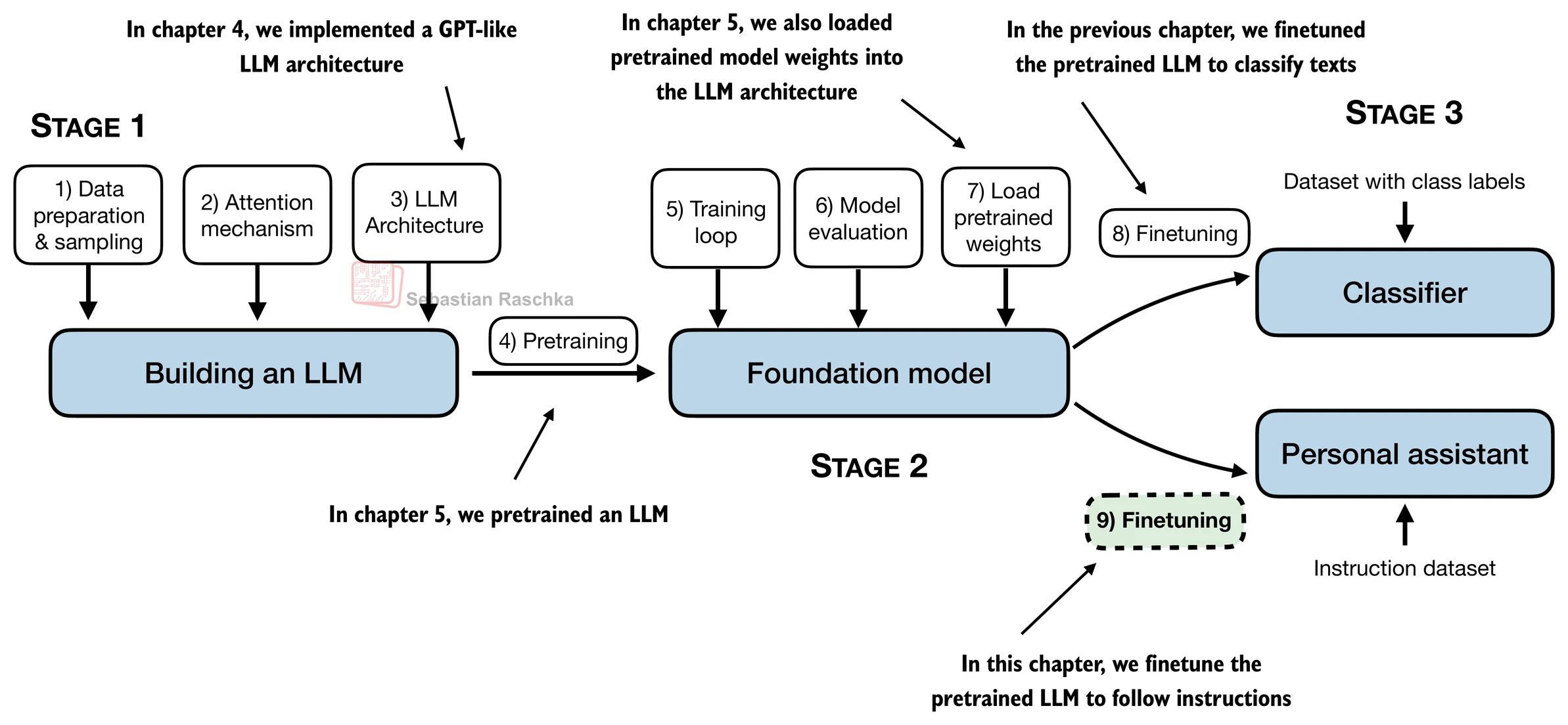
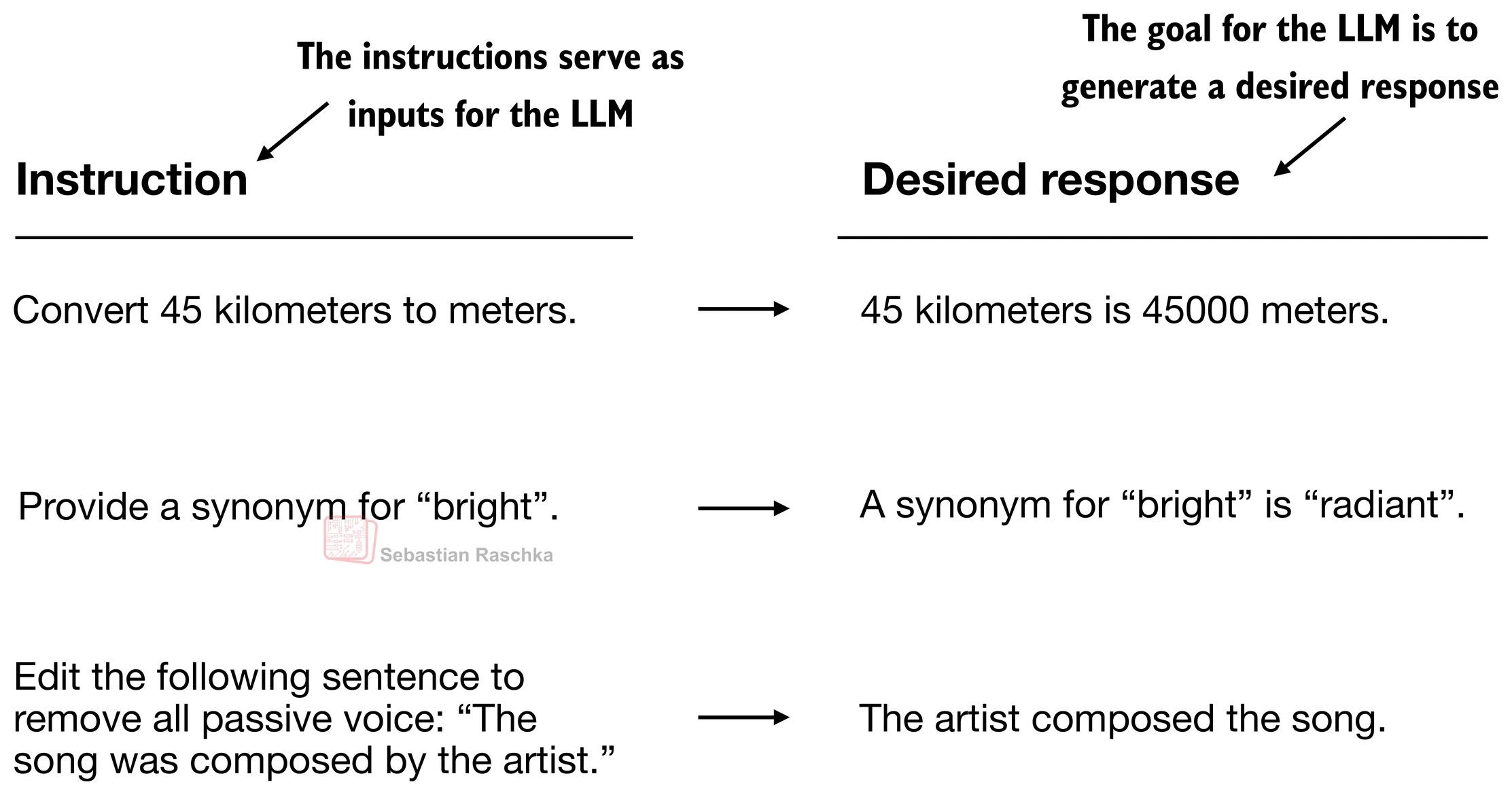
In previous chapter, we saw that pretraining an LLM involves a training procedure where it learns to generate one word at a time. Hence, a pretrained LLM is good at text completion, but it is not good at following instructions. In this chapter, we teach the LLM to follow instructions better.

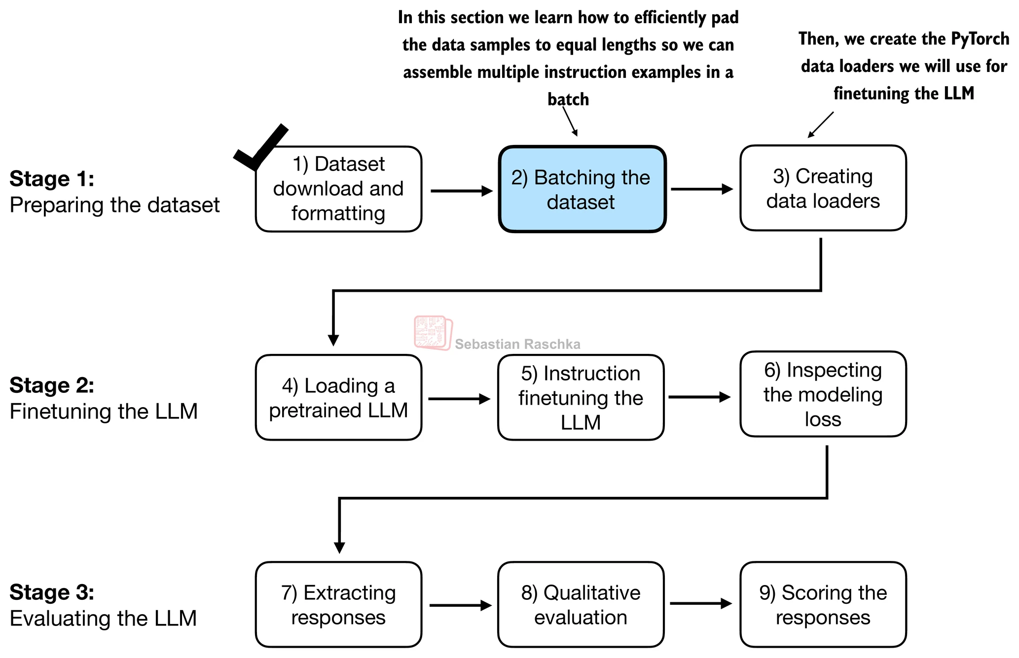
The topics covered in this chapter are summarized in the figure below:

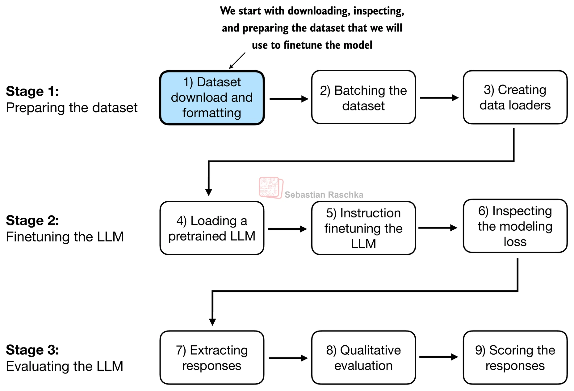
Stage 1: Preparing a dataset for supervised instruction finetuning¶

Download and format dataset¶

We will work with an instruction dataset Dr. Raschka prepared for this chapter.

import json
import os
import requests


def download_and_load_file(file_path, url):
    if not os.path.exists(file_path):
        response = requests.get(url, timeout=30)
        response.raise_for_status()
        text_data = response.text
        with open(file_path, "w", encoding="utf-8") as file:
            file.write(text_data)

    with open(file_path, "r", encoding="utf-8") as file:
        data = json.load(file)

    return data

file_path = "instruction-data.json"
url = (
    "https://raw.githubusercontent.com/rasbt/LLMs-from-scratch"
    "/main/ch07/01_main-chapter-code/instruction-data.json"
)

data = download_and_load_file(file_path, url)
print("Number of entries:", len(data))

Number of entries: 1100

Each item in the data list we loaded from the JSON file above is a dictionary in the following form

print("Example entry:\n", data[50])

Example entry:
 {'instruction': 'Identify the correct spelling of the following word.', 'input': 'Ocassion', 'output': "The correct spelling is 'Occasion.'"}

Note that the 'input' field can be empty:

print("Another example entry:\n", data[999])

Another example entry:
 {'instruction': "What is an antonym of 'complicated'?", 'input': '', 'output': "An antonym of 'complicated' is 'simple'."}

Instruction finetuning is often referred to as “supervised instruction finetuning” because it involves training a model on a dataset where the input-output pairs are explicitly provided.

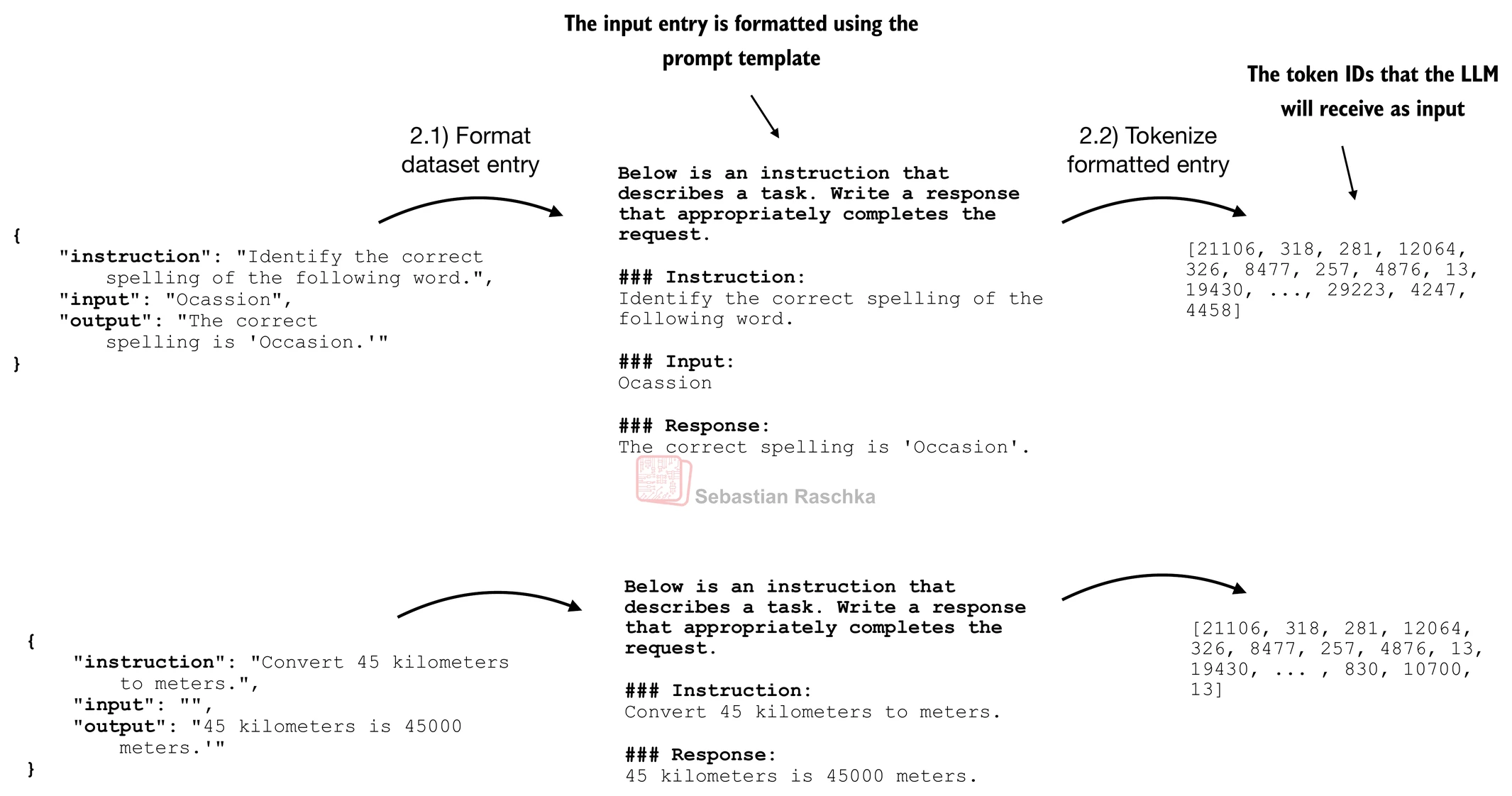
There are different ways to format the entries as inputs to the LLM; the figure below illustrates two example formats that were used for training the Alpaca (https://crfm.stanford.edu/2023/03/13/alpaca.html) and Phi-3 (https://arxiv.org/abs/2404.14219) LLMs, respectively

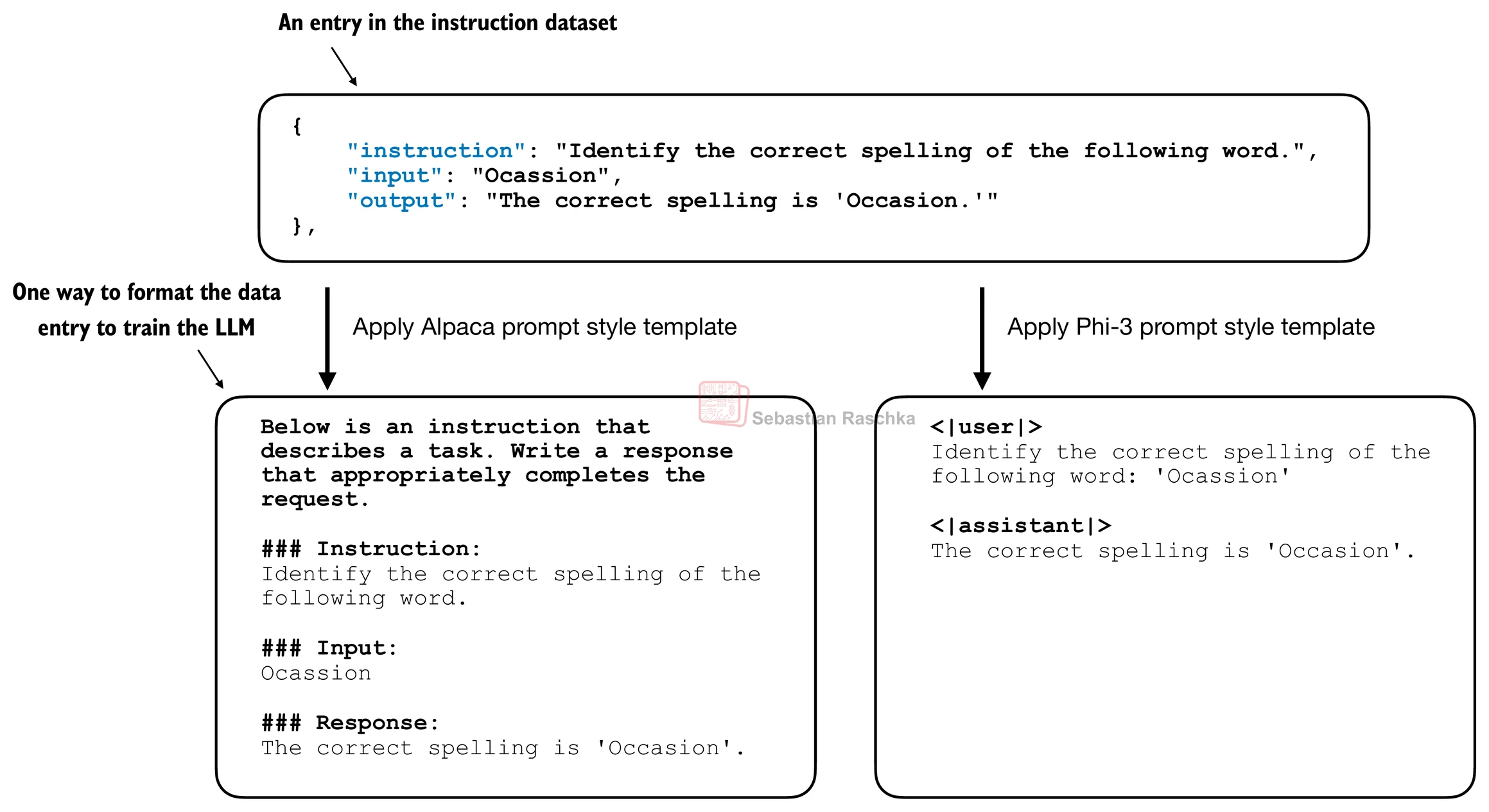
In this chapter, we use Alpaca-style prompt formatting, which was the original prompt template for instruction finetuning.

Below, we format the input that we will pass as input to the LLM.

def format_input(entry):
    instruction_text = (
        f"Below is an instruction that describes a task. "
        f"Write a response that appropriately completes the request."
        f"\n\n### Instruction:\n{entry['instruction']}"
    )

    input_text = f"\n\n### Input:\n{entry['input']}" if entry["input"] else ""

    return instruction_text + input_text

A formatted response with input field looks like as shown below:

model_input = format_input(data[50])
desired_response = f"\n\n### Response:\n{data[50]['output']}"

print(model_input + desired_response)

Below is an instruction that describes a task. Write a response that appropriately completes the request.

### Instruction:
Identify the correct spelling of the following word.

### Input:
Ocassion

### Response:
The correct spelling is 'Occasion.'

Below is a formatted response without an input field.

model_input = format_input(data[999])
desired_response = f"\n\n### Response:\n{data[999]['output']}"

print(model_input + desired_response)

Below is an instruction that describes a task. Write a response that appropriately completes the request.

### Instruction:
What is an antonym of 'complicated'?

### Response:
An antonym of 'complicated' is 'simple'.

Lastly, before we prepare the PyTorch data loaders in the next section, we divide the dataset into a training, validation, and test set.

train_portion = int(len(data) * 0.85)  # 85% for training
test_portion = int(len(data) * 0.1)    # 10% for testing
val_portion = len(data) - train_portion - test_portion  # Remaining 5% for validation

train_data = data[:train_portion]
test_data = data[train_portion:train_portion + test_portion]
val_data = data[train_portion + test_portion:]

print("Training set length:", len(train_data))
print("Validation set length:", len(val_data))
print("Test set length:", len(test_data))

Training set length: 935
Validation set length: 55
Test set length: 110

Organize data into training batches¶

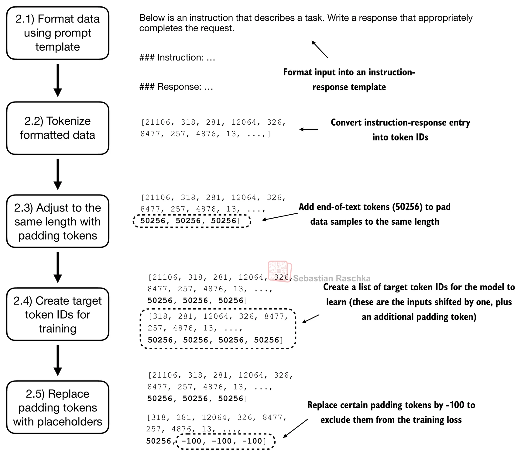
We tackle this dataset batching in several steps, as summarized in the figure below.

First, we implement an InstructionDataset class that pre-tokenizes all inputs in the dataset.

import torch
from torch.utils.data import Dataset


class InstructionDataset(Dataset):
    def __init__(self, data, tokenizer):
        self.data = data

        # Pre-tokenize texts
        self.encoded_texts = []
        for entry in data:
            instruction_plus_input = format_input(entry)
            response_text = f"\n\n### Response:\n{entry['output']}"
            full_text = instruction_plus_input + response_text
            self.encoded_texts.append(
                tokenizer.encode(full_text)
            )

    def __getitem__(self, index):
        return self.encoded_texts[index]

    def __len__(self):
        return len(self.data)

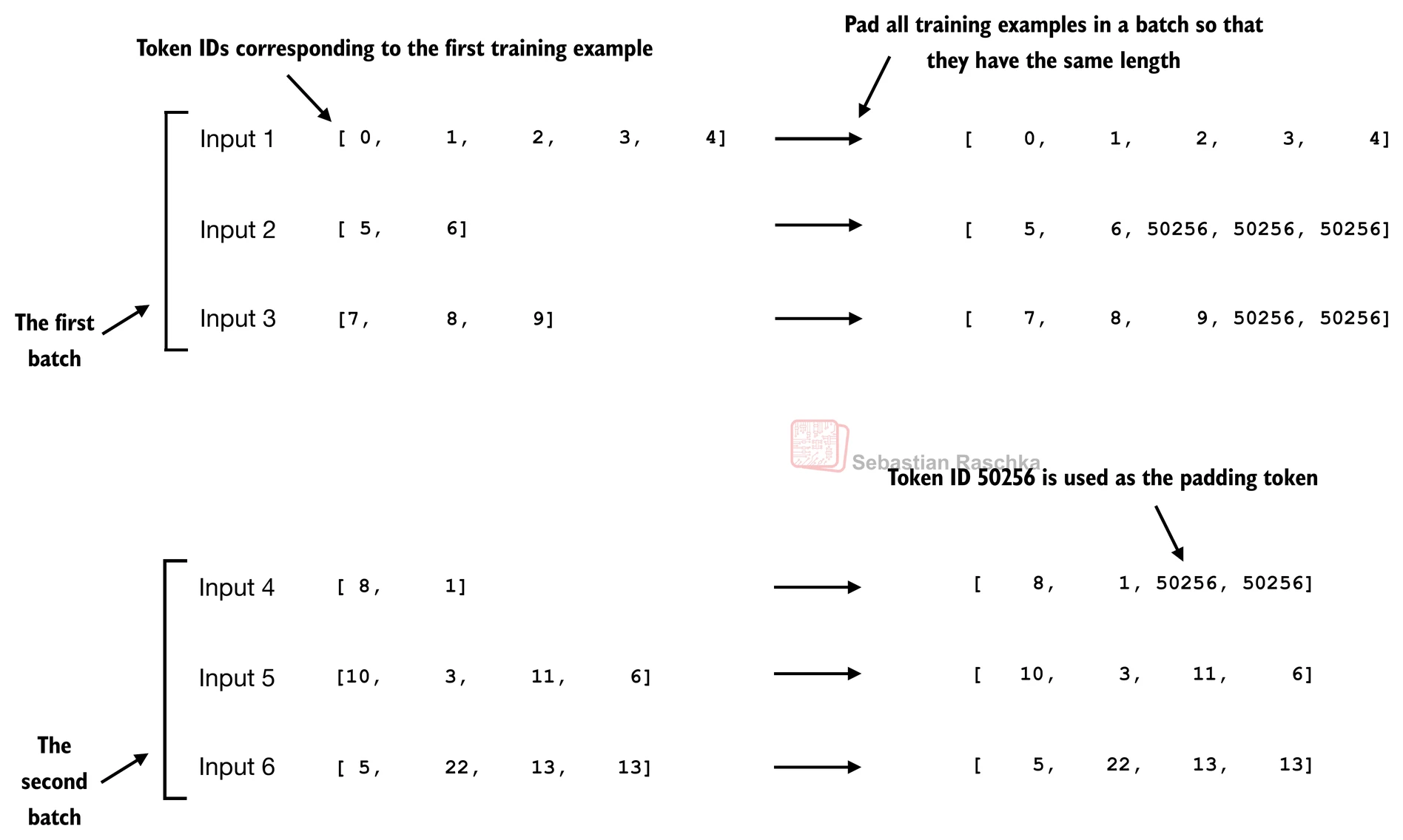
Similar to previous chapter, we want to collect multiple training examples in a batch to accelerate training; this requires padding all inputs to a similar length. Here, we use the <|endoftext|> token as a padding token.

import tiktoken
tokenizer = tiktoken.get_encoding("gpt2")

print(tokenizer.encode("<|endoftext|>", allowed_special={"<|endoftext|>"}))

[50256]

Here, we develop a custom “collate” function that we can pass to the data loader, which pads the training examples in each batch to have the same length (but different batches can have different lengths).

def custom_collate_draft_1(
    batch,
    pad_token_id=50256,
    device="cpu"
):
    # Find the longest sequence in the batch
    # and increase the max length by +1, which will add one extra
    # padding token below
    batch_max_length = max(len(item)+1 for item in batch)

    # Pad and prepare inputs
    inputs_lst = []

    for item in batch:
        new_item = item.copy()
        # Add an <|endoftext|> token
        new_item += [pad_token_id]
        # Pad sequences to batch_max_length
        padded = (
            new_item + [pad_token_id] *
            (batch_max_length - len(new_item))
        )
        # Via padded[:-1], we remove the extra padded token
        # that has been added via the +1 setting in batch_max_length
        # (the extra padding token will be relevant in later codes)
        inputs = torch.tensor(padded[:-1])
        inputs_lst.append(inputs)

    # Convert list of inputs to tensor and transfer to target device
    inputs_tensor = torch.stack(inputs_lst).to(device)
    return inputs_tensor

inputs_1 = [0, 1, 2, 3, 4]
inputs_2 = [5, 6]
inputs_3 = [7, 8, 9]

batch = (
    inputs_1,
    inputs_2,
    inputs_3
)

print(custom_collate_draft_1(batch))

tensor([[    0,     1,     2,     3,     4],
        [    5,     6, 50256, 50256, 50256],
        [    7,     8,     9, 50256, 50256]])

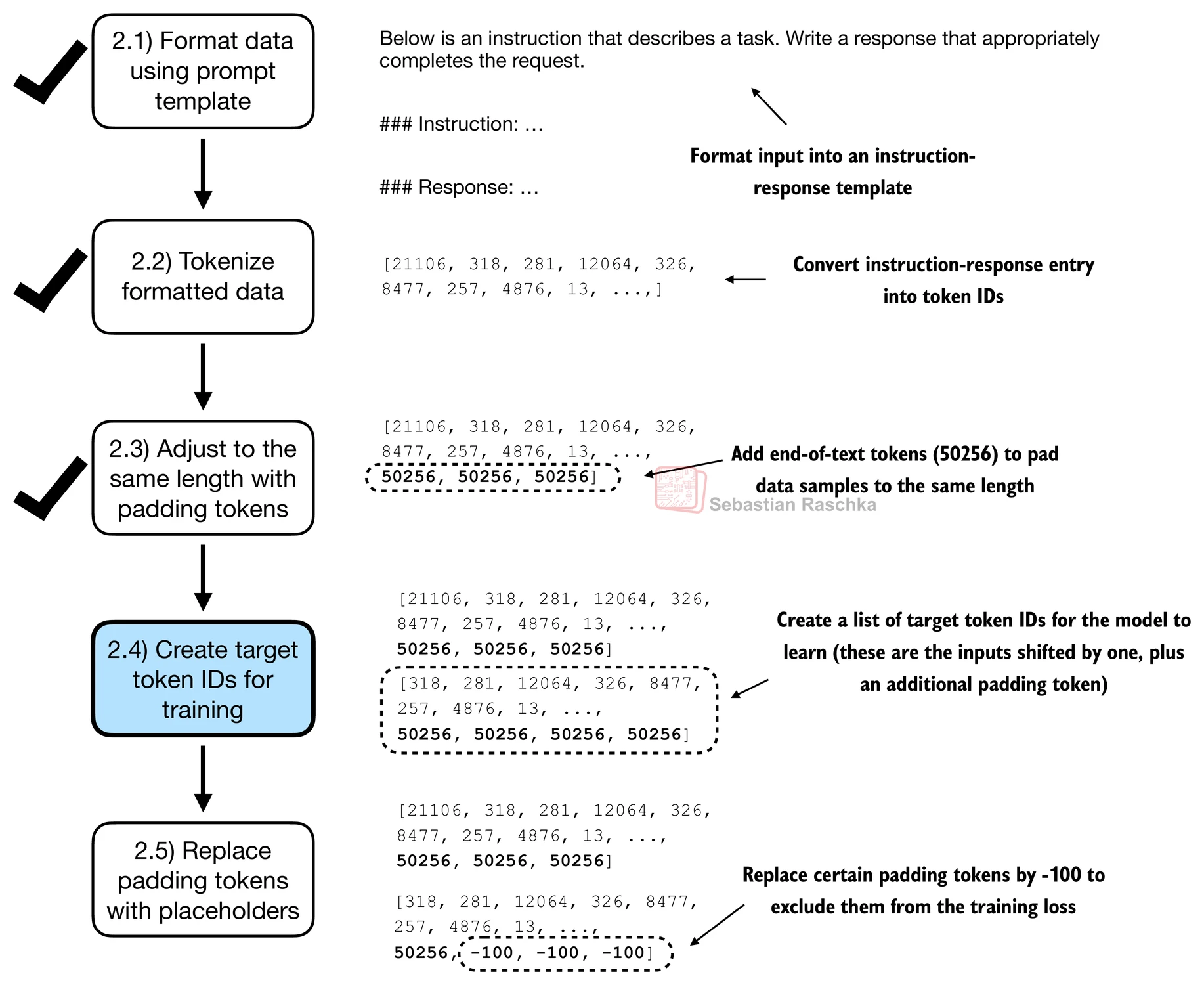
Above, we only returned the inputs to the LLM; however, for LLM training, we also need the target values. Similar to pretraining an LLM, the targets are the inputs shifted by 1 position to the right, so the LLM learns to predict the next token.

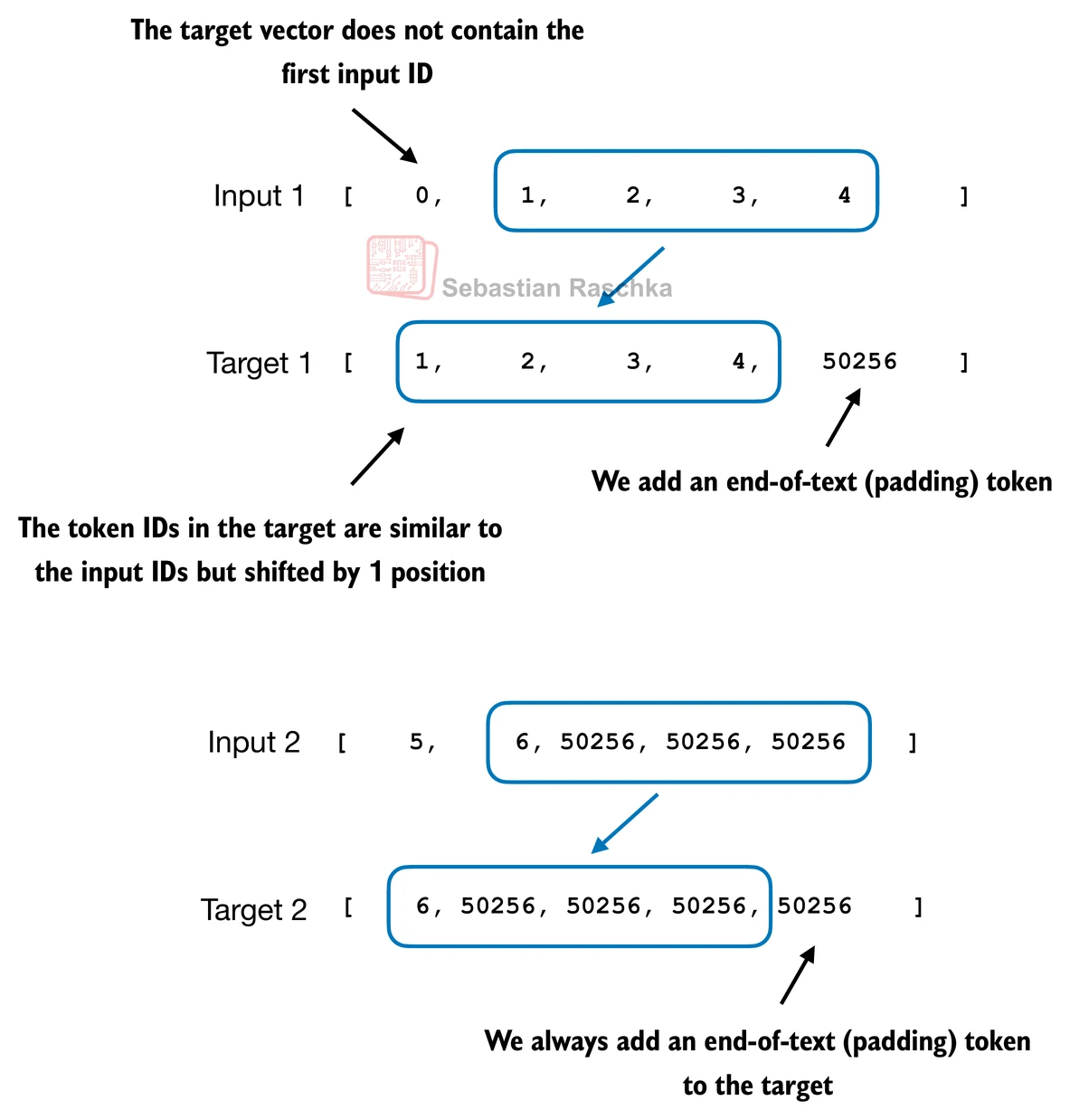
def custom_collate_draft_2(
    batch,
    pad_token_id=50256,
    device="cpu"
):
    # Find the longest sequence in the batch
    batch_max_length = max(len(item)+1 for item in batch)

    # Pad and prepare inputs
    inputs_lst, targets_lst = [], []

    for item in batch:
        new_item = item.copy()
        # Add an <|endoftext|> token
        new_item += [pad_token_id]
        # Pad sequences to max_length
        padded = (
            new_item + [pad_token_id] *
            (batch_max_length - len(new_item))
        )
        inputs = torch.tensor(padded[:-1])  # Truncate the last token for inputs
        targets = torch.tensor(padded[1:])  # Shift +1 to the right for targets
        inputs_lst.append(inputs)
        targets_lst.append(targets)

    # Convert list of inputs to tensor and transfer to target device
    inputs_tensor = torch.stack(inputs_lst).to(device)
    targets_tensor = torch.stack(targets_lst).to(device)
    return inputs_tensor, targets_tensor

inputs, targets = custom_collate_draft_2(batch)
print(inputs)
print(targets)

tensor([[    0,     1,     2,     3,     4],
        [    5,     6, 50256, 50256, 50256],
        [    7,     8,     9, 50256, 50256]])
tensor([[    1,     2,     3,     4, 50256],
        [    6, 50256, 50256, 50256, 50256],
        [    8,     9, 50256, 50256, 50256]])

Next, we introduce an ignore_index value to replace all padding token IDs with a new value ; the purpose of this ignore_index is that we can ignore padding values in the loss function.

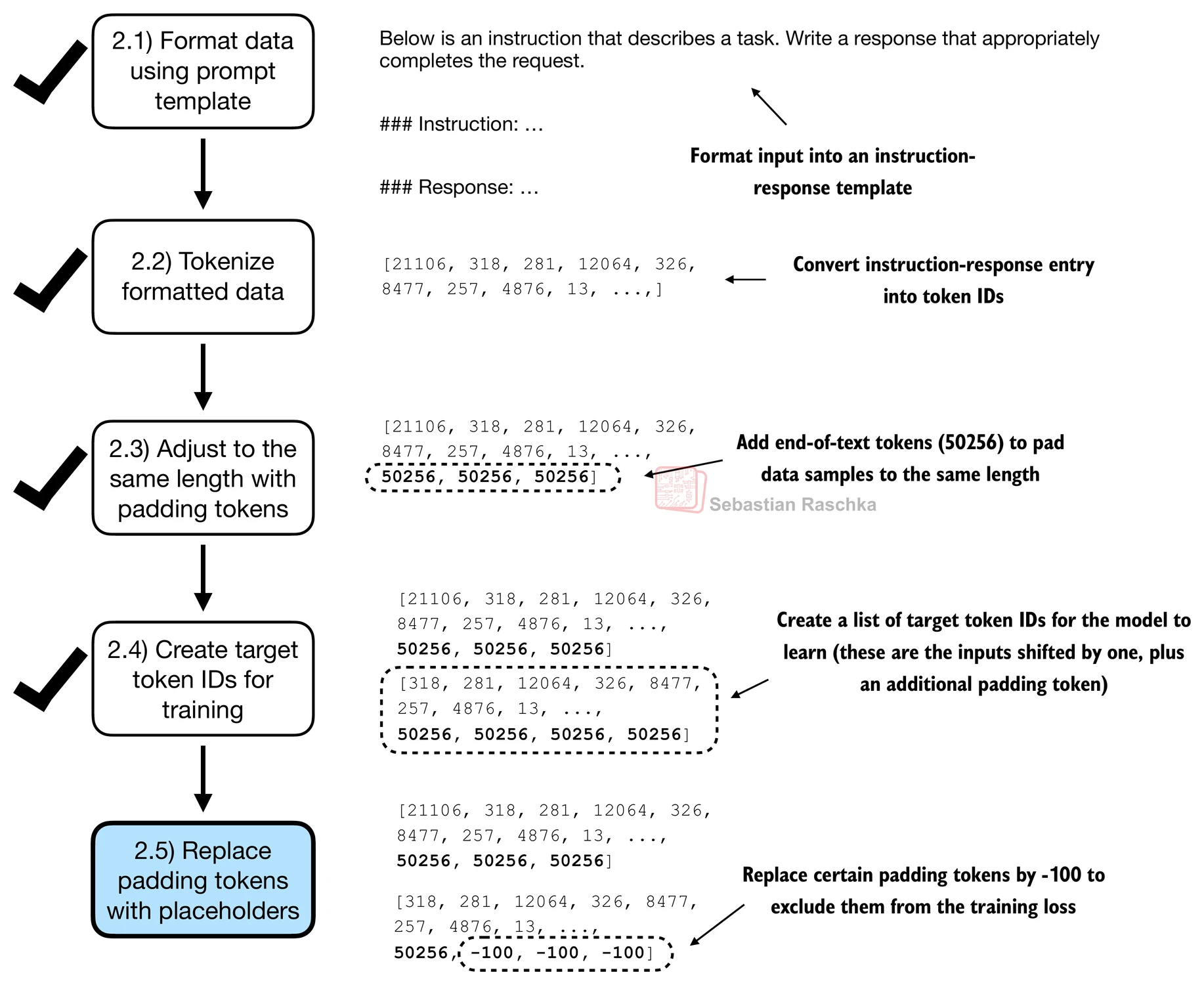
Concretely, this means that we replace the token IDs corresponding to 50256 with -100 as illustrated below:

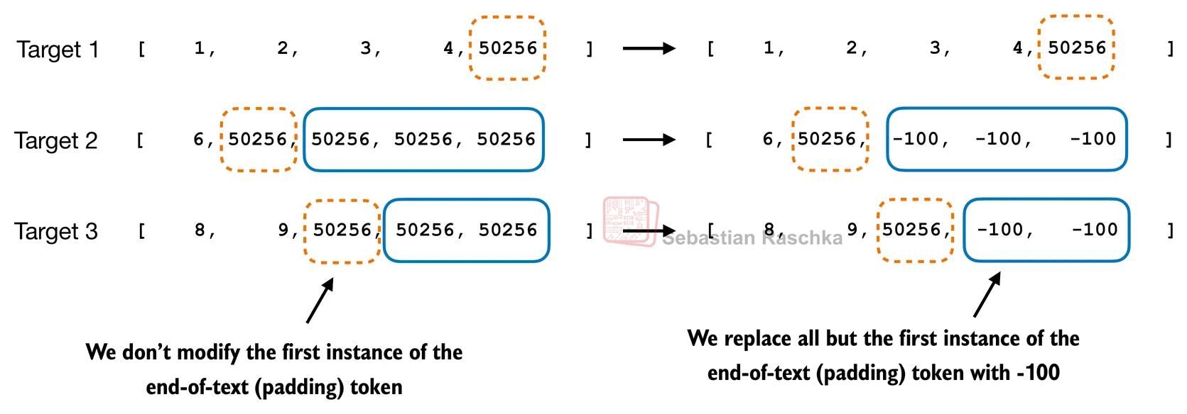
In addition, we also introduce the allowed_max_length in case we want to limit the length of the samples ; this will be useful if you plan to work with your own datasets that are longer than the 1024 token context size supported by the GPT-2 model.

def custom_collate_fn(
    batch,
    pad_token_id=50256,
    ignore_index=-100,
    allowed_max_length=None,
    device="cpu"
):
    # Find the longest sequence in the batch
    batch_max_length = max(len(item)+1 for item in batch)

    # Pad and prepare inputs and targets
    inputs_lst, targets_lst = [], []

    for item in batch:
        new_item = item.copy()
        # Add an <|endoftext|> token
        new_item += [pad_token_id]
        # Pad sequences to max_length
        padded = (
            new_item + [pad_token_id] *
            (batch_max_length - len(new_item))
        )
        inputs = torch.tensor(padded[:-1])  # Truncate the last token for inputs
        targets = torch.tensor(padded[1:])  # Shift +1 to the right for targets

        # New: Replace all but the first padding tokens in targets by ignore_index
        mask = targets == pad_token_id
        indices = torch.nonzero(mask).squeeze()
        if indices.numel() > 1:
            targets[indices[1:]] = ignore_index

        # New: Optionally truncate to maximum sequence length
        if allowed_max_length is not None:
            inputs = inputs[:allowed_max_length]
            targets = targets[:allowed_max_length]

        inputs_lst.append(inputs)
        targets_lst.append(targets)

    # Convert list of inputs and targets to tensors and transfer to target device
    inputs_tensor = torch.stack(inputs_lst).to(device)
    targets_tensor = torch.stack(targets_lst).to(device)

    return inputs_tensor, targets_tensor

inputs, targets = custom_collate_fn(batch)
print(inputs)
print(targets)

tensor([[    0,     1,     2,     3,     4],
        [    5,     6, 50256, 50256, 50256],
        [    7,     8,     9, 50256, 50256]])
tensor([[    1,     2,     3,     4, 50256],
        [    6, 50256,  -100,  -100,  -100],
        [    8,     9, 50256,  -100,  -100]])

Let’s see what this replacement by -100 accomplishes. For illustration purposes, let’s assume we have a small classification task with 2 class labels, 0 and 1. If we have the following logits values (outputs of the last layer of the model), we calculate the following loss/

logits_1 = torch.tensor(
    [[-1.0, 1.0],  # 1st training example
     [-0.5, 1.5]]  # 2nd training example
)
targets_1 = torch.tensor([0, 1])


loss_1 = torch.nn.functional.cross_entropy(logits_1, targets_1)
print(loss_1)

tensor(1.1269)

Now, adding one more training example will, as expected, influence the loss.

logits_2 = torch.tensor(
    [[-1.0, 1.0],
     [-0.5, 1.5],
     [-0.5, 1.5]]  # New 3rd training example
)
targets_2 = torch.tensor([0, 1, 1])

loss_2 = torch.nn.functional.cross_entropy(logits_2, targets_2)
print(loss_2)

tensor(0.7936)

Let’s see what happens if we replace the class label of one of the examples with -100.

targets_3 = torch.tensor([0, 1, -100])

loss_3 = torch.nn.functional.cross_entropy(logits_2, targets_3)
print(loss_3)
print("loss_1 == loss_3:", loss_1 == loss_3)

tensor(1.1269)
loss_1 == loss_3: tensor(True)

As we can see, the resulting loss on these 3 training examples is the same as the loss we calculated from the 2 training examples, which means that the cross-entropy loss function ignored the training example with the -100 label.

By default, PyTorch has the cross_entropy(..., ignore_index=-100) setting to ignore examples corresponding to the label -100.
Using this -100 ignore_index, we can ignore the additional end-of-text (padding) tokens in the batches that we used to pad the training examples to equal length
However, we don’t want to ignore the first instance of the end-of-text (padding) token (50256) because it can help signal to the LLM when the response is complete.

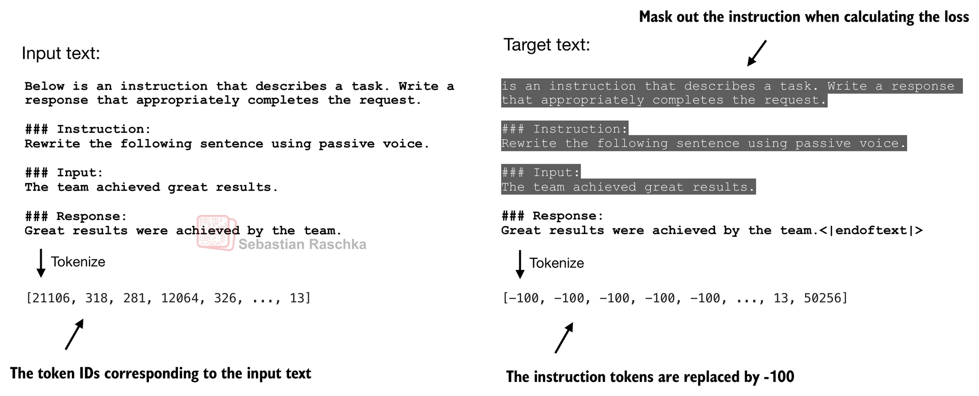
In practice, it is also common to mask out the target token IDs that correspond to the instruction , as illustrated in the figure below (this is a recommended reader exercise after completing the chapter).

Create data loaders¶

In this section, we use the InstructionDataset class and custom_collate_fn function to instantiate the training, validation, and test data loaders.

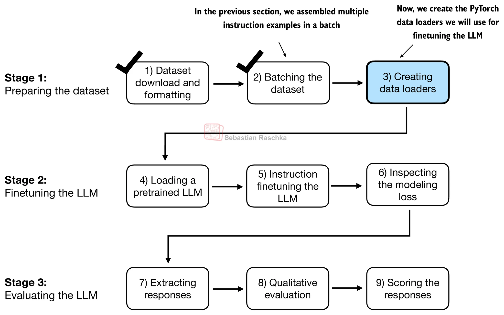
Another additional detail of the previous custom_collate_fn function is that we now directly move the data to the target device (e.g., GPU) instead of doing it in the main training loop, which improves efficiency because it can be carried out as a background process when we use the custom_collate_fn as part of the data loader.

Using the partial function from Python’s functools standard library, we create a new function with the device argument of the original function pre-filled.

if torch.cuda.is_available():
    device = torch.device("cuda")
elif torch.backends.mps.is_available():
    # Use PyTorch 2.9 or newer for stable mps results
    major, minor = map(int, torch.__version__.split(".")[:2])
    if (major, minor) >= (2, 9):
        device = torch.device("mps")
    else:
        device = torch.device("cpu")
else:
    device = torch.device("cpu")

print("Device:", device)

Device: cuda

from functools import partial

customized_collate_fn = partial(
    custom_collate_fn,
    device=device,
    allowed_max_length=1024
)

Next, we instantiate the data loaders similar to previous chapters, except that we now provide our own collate function for the batching process.

from torch.utils.data import DataLoader


num_workers = 0
batch_size = 8

torch.manual_seed(123)

train_dataset = InstructionDataset(train_data, tokenizer)
train_loader = DataLoader(
    train_dataset,
    batch_size=batch_size,
    collate_fn=customized_collate_fn,
    shuffle=True,
    drop_last=True,
    num_workers=num_workers
)

val_dataset = InstructionDataset(val_data, tokenizer)
val_loader = DataLoader(
    val_dataset,
    batch_size=batch_size,
    collate_fn=customized_collate_fn,
    shuffle=False,
    drop_last=False,
    num_workers=num_workers
)

test_dataset = InstructionDataset(test_data, tokenizer)
test_loader = DataLoader(
    test_dataset,
    batch_size=batch_size,
    collate_fn=customized_collate_fn,
    shuffle=False,
    drop_last=False,
    num_workers=num_workers
)

Let’s see what the dimensions of the resulting input and target batches look like:

print("Train loader:")
for inputs, targets in train_loader:
    print(inputs.shape, targets.shape)

Train loader:
torch.Size([8, 61]) torch.Size([8, 61])
torch.Size([8, 76]) torch.Size([8, 76])
torch.Size([8, 73]) torch.Size([8, 73])
torch.Size([8, 68]) torch.Size([8, 68])
torch.Size([8, 65]) torch.Size([8, 65])
torch.Size([8, 72]) torch.Size([8, 72])
torch.Size([8, 80]) torch.Size([8, 80])
torch.Size([8, 67]) torch.Size([8, 67])
torch.Size([8, 62]) torch.Size([8, 62])
torch.Size([8, 75]) torch.Size([8, 75])
torch.Size([8, 62]) torch.Size([8, 62])
torch.Size([8, 68]) torch.Size([8, 68])
torch.Size([8, 67]) torch.Size([8, 67])
torch.Size([8, 77]) torch.Size([8, 77])
torch.Size([8, 69]) torch.Size([8, 69])
torch.Size([8, 79]) torch.Size([8, 79])
torch.Size([8, 71]) torch.Size([8, 71])
torch.Size([8, 66]) torch.Size([8, 66])
torch.Size([8, 83]) torch.Size([8, 83])
torch.Size([8, 68]) torch.Size([8, 68])
torch.Size([8, 80]) torch.Size([8, 80])
torch.Size([8, 71]) torch.Size([8, 71])
torch.Size([8, 69]) torch.Size([8, 69])
torch.Size([8, 65]) torch.Size([8, 65])
torch.Size([8, 68]) torch.Size([8, 68])
torch.Size([8, 60]) torch.Size([8, 60])
torch.Size([8, 59]) torch.Size([8, 59])
torch.Size([8, 69]) torch.Size([8, 69])
torch.Size([8, 63]) torch.Size([8, 63])
torch.Size([8, 65]) torch.Size([8, 65])
torch.Size([8, 76]) torch.Size([8, 76])
torch.Size([8, 66]) torch.Size([8, 66])
torch.Size([8, 71]) torch.Size([8, 71])
torch.Size([8, 91]) torch.Size([8, 91])
torch.Size([8, 65]) torch.Size([8, 65])
torch.Size([8, 64]) torch.Size([8, 64])
torch.Size([8, 67]) torch.Size([8, 67])
torch.Size([8, 66]) torch.Size([8, 66])
torch.Size([8, 64]) torch.Size([8, 64])
torch.Size([8, 65]) torch.Size([8, 65])
torch.Size([8, 75]) torch.Size([8, 75])
torch.Size([8, 89]) torch.Size([8, 89])
torch.Size([8, 59]) torch.Size([8, 59])
torch.Size([8, 88]) torch.Size([8, 88])
torch.Size([8, 83]) torch.Size([8, 83])
torch.Size([8, 83]) torch.Size([8, 83])
torch.Size([8, 70]) torch.Size([8, 70])
torch.Size([8, 65]) torch.Size([8, 65])
torch.Size([8, 74]) torch.Size([8, 74])
torch.Size([8, 76]) torch.Size([8, 76])
torch.Size([8, 67]) torch.Size([8, 67])
torch.Size([8, 75]) torch.Size([8, 75])
torch.Size([8, 83]) torch.Size([8, 83])
torch.Size([8, 69]) torch.Size([8, 69])
torch.Size([8, 67]) torch.Size([8, 67])
torch.Size([8, 60]) torch.Size([8, 60])
torch.Size([8, 60]) torch.Size([8, 60])
torch.Size([8, 66]) torch.Size([8, 66])
torch.Size([8, 80]) torch.Size([8, 80])
torch.Size([8, 71]) torch.Size([8, 71])
torch.Size([8, 61]) torch.Size([8, 61])
torch.Size([8, 58]) torch.Size([8, 58])
torch.Size([8, 71]) torch.Size([8, 71])
torch.Size([8, 67]) torch.Size([8, 67])
torch.Size([8, 68]) torch.Size([8, 68])
torch.Size([8, 63]) torch.Size([8, 63])
torch.Size([8, 87]) torch.Size([8, 87])
torch.Size([8, 68]) torch.Size([8, 68])
torch.Size([8, 64]) torch.Size([8, 64])
torch.Size([8, 68]) torch.Size([8, 68])
torch.Size([8, 71]) torch.Size([8, 71])
torch.Size([8, 68]) torch.Size([8, 68])
torch.Size([8, 71]) torch.Size([8, 71])
torch.Size([8, 61]) torch.Size([8, 61])
torch.Size([8, 65]) torch.Size([8, 65])
torch.Size([8, 67]) torch.Size([8, 67])
torch.Size([8, 65]) torch.Size([8, 65])
torch.Size([8, 64]) torch.Size([8, 64])
torch.Size([8, 60]) torch.Size([8, 60])
torch.Size([8, 72]) torch.Size([8, 72])
torch.Size([8, 64]) torch.Size([8, 64])
torch.Size([8, 70]) torch.Size([8, 70])
torch.Size([8, 57]) torch.Size([8, 57])
torch.Size([8, 72]) torch.Size([8, 72])
torch.Size([8, 64]) torch.Size([8, 64])
torch.Size([8, 68]) torch.Size([8, 68])
torch.Size([8, 62]) torch.Size([8, 62])
torch.Size([8, 74]) torch.Size([8, 74])
torch.Size([8, 80]) torch.Size([8, 80])
torch.Size([8, 68]) torch.Size([8, 68])
torch.Size([8, 70]) torch.Size([8, 70])
torch.Size([8, 91]) torch.Size([8, 91])
torch.Size([8, 61]) torch.Size([8, 61])
torch.Size([8, 66]) torch.Size([8, 66])
torch.Size([8, 80]) torch.Size([8, 80])
torch.Size([8, 81]) torch.Size([8, 81])
torch.Size([8, 74]) torch.Size([8, 74])
torch.Size([8, 82]) torch.Size([8, 82])
torch.Size([8, 63]) torch.Size([8, 63])
torch.Size([8, 83]) torch.Size([8, 83])
torch.Size([8, 68]) torch.Size([8, 68])
torch.Size([8, 67]) torch.Size([8, 67])
torch.Size([8, 77]) torch.Size([8, 77])
torch.Size([8, 91]) torch.Size([8, 91])
torch.Size([8, 64]) torch.Size([8, 64])
torch.Size([8, 61]) torch.Size([8, 61])
torch.Size([8, 75]) torch.Size([8, 75])
torch.Size([8, 64]) torch.Size([8, 64])
torch.Size([8, 66]) torch.Size([8, 66])
torch.Size([8, 78]) torch.Size([8, 78])
torch.Size([8, 66]) torch.Size([8, 66])
torch.Size([8, 64]) torch.Size([8, 64])
torch.Size([8, 83]) torch.Size([8, 83])
torch.Size([8, 66]) torch.Size([8, 66])
torch.Size([8, 74]) torch.Size([8, 74])
torch.Size([8, 69]) torch.Size([8, 69])

As we can see based on the output above, all batches have a batch size of 8 but a different length. Let’s also double-check that the inputs contain the <|endoftext|> padding tokens corresponding to token ID 50256 by printing the contents of the first training example in the inputs batch.

print(inputs[0])

tensor([21106,   318,   281, 12064,   326,  8477,   257,  4876,    13, 19430,
          257,  2882,   326, 20431, 32543,   262,  2581,    13,   198,   198,
        21017, 46486,    25,   198, 30003,  6525,   262,  6827,  1262,   257,
          985,   576,    13,   198,   198, 21017, 23412,    25,   198,   464,
         5156,   318,   845, 13779,    13,   198,   198, 21017, 18261,    25,
          198,   464,  5156,   318,   355, 13779,   355,   257,  4936,    13,
        50256, 50256, 50256, 50256, 50256, 50256, 50256, 50256, 50256],
       device='cuda:0')

Similarly, we visually double-check that the targets contain the -100 placeholder tokens.

print(targets[0])

tensor([  318,   281, 12064,   326,  8477,   257,  4876,    13, 19430,   257,
         2882,   326, 20431, 32543,   262,  2581,    13,   198,   198, 21017,
        46486,    25,   198, 30003,  6525,   262,  6827,  1262,   257,   985,
          576,    13,   198,   198, 21017, 23412,    25,   198,   464,  5156,
          318,   845, 13779,    13,   198,   198, 21017, 18261,    25,   198,
          464,  5156,   318,   355, 13779,   355,   257,  4936,    13, 50256,
         -100,  -100,  -100,  -100,  -100,  -100,  -100,  -100,  -100],
       device='cuda:0')

Stage 2: Finetuning LLM¶

Load a pretrained LLM¶

Here, we load a pretrained GPT model using the same code that we used before.

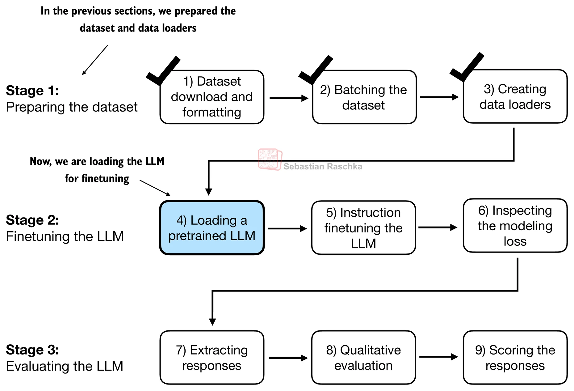
However, instead of loading the smallest 124 million parameter model, we load the medium version with 355 million parameters since the 124 million model is too small for achieving qualitatively reasonable results via instruction finetuning.

# Download the file from my github
# Note that we save the file in the temporary folder of Google Colab,
# it will dispear once you close the session.
!wget -O /content/previous_chapters.py https://raw.githubusercontent.com/brianjalaian/CAP6606_ML_ISR/main/modules/02-LLM/06-finetuning_instruction/data/previous_chapters.py

!wget -O /content/gpt_download.py https://raw.githubusercontent.com/brianjalaian/CAP6606_ML_ISR/main/modules/02-LLM/06-finetuning_instruction/data/gpt_download.py

--2026-05-20 03:16:53--  https://raw.githubusercontent.com/brianjalaian/CAP6606_ML_ISR/main/modules/02-LLM/06-finetuning_instruction/data/previous_chapters.py
Resolving raw.githubusercontent.com (raw.githubusercontent.com)... 185.199.108.133, 185.199.109.133, 185.199.110.133, ...
Connecting to raw.githubusercontent.com (raw.githubusercontent.com)|185.199.108.133|:443... connected.
HTTP request sent, awaiting response... 200 OK
Length: 18236 (18K) [text/plain]
Saving to: ‘/content/previous_chapters.py’

/content/previous_c 100%[===================>]  17.81K  --.-KB/s    in 0.001s  

2026-05-20 03:16:53 (20.9 MB/s) - ‘/content/previous_chapters.py’ saved [18236/18236]

--2026-05-20 03:16:53--  https://raw.githubusercontent.com/brianjalaian/CAP6606_ML_ISR/main/modules/02-LLM/06-finetuning_instruction/data/gpt_download.py
Resolving raw.githubusercontent.com (raw.githubusercontent.com)... 185.199.108.133, 185.199.111.133, 185.199.109.133, ...
Connecting to raw.githubusercontent.com (raw.githubusercontent.com)|185.199.108.133|:443... connected.
HTTP request sent, awaiting response... 200 OK
Length: 4687 (4.6K) [text/plain]
Saving to: ‘/content/gpt_download.py’

/content/gpt_downlo 100%[===================>]   4.58K  --.-KB/s    in 0s      

2026-05-20 03:16:54 (58.7 MB/s) - ‘/content/gpt_download.py’ saved [4687/4687]

from gpt_download import download_and_load_gpt2
from previous_chapters import GPTModel, load_weights_into_gpt


BASE_CONFIG = {
    "vocab_size": 50257,     # Vocabulary size
    "context_length": 1024,  # Context length
    "drop_rate": 0.0,        # Dropout rate
    "qkv_bias": True         # Query-key-value bias
}

model_configs = {
    "gpt2-small (124M)": {"emb_dim": 768, "n_layers": 12, "n_heads": 12},
    "gpt2-medium (355M)": {"emb_dim": 1024, "n_layers": 24, "n_heads": 16},
    "gpt2-large (774M)": {"emb_dim": 1280, "n_layers": 36, "n_heads": 20},
    "gpt2-xl (1558M)": {"emb_dim": 1600, "n_layers": 48, "n_heads": 25},
}

CHOOSE_MODEL = "gpt2-medium (355M)"

BASE_CONFIG.update(model_configs[CHOOSE_MODEL])

model_size = CHOOSE_MODEL.split(" ")[-1].lstrip("(").rstrip(")")
settings, params = download_and_load_gpt2(
    model_size=model_size,
    models_dir="gpt2"
)

model = GPTModel(BASE_CONFIG)
load_weights_into_gpt(model, params)
model.eval();

checkpoint: 100%|██████████| 77.0/77.0 [00:00<00:00, 62.8kiB/s]
encoder.json: 100%|██████████| 1.04M/1.04M [00:00<00:00, 2.60MiB/s]
hparams.json: 100%|██████████| 91.0/91.0 [00:00<00:00, 205kiB/s]
model.ckpt.data-00000-of-00001: 100%|██████████| 1.42G/1.42G [01:59<00:00, 11.9MiB/s]
model.ckpt.index: 100%|██████████| 10.4k/10.4k [00:00<00:00, 22.1MiB/s]
model.ckpt.meta: 100%|██████████| 927k/927k [00:00<00:00, 3.13MiB/s]
vocab.bpe: 100%|██████████| 456k/456k [00:00<00:00, 1.52MiB/s]

Before we start finetuning the model in the next section, let’s see how it performs on one of the validation tasks.

Spoil alert: Before instruction-tuning, the model can’t follow instruction well.

torch.manual_seed(123)

input_text = format_input(val_data[0])
print(input_text)

Below is an instruction that describes a task. Write a response that appropriately completes the request.

### Instruction:
Convert the active sentence to passive: 'The chef cooks the meal every day.'

Note that the following generate function we used in previous chapters returns the combined input and output text, which was convenient in the previous section for creating legible text.

from previous_chapters import (
    generate,
    text_to_token_ids,
    token_ids_to_text
)


token_ids = generate(
    model=model,
    idx=text_to_token_ids(input_text, tokenizer),
    max_new_tokens=35,
    context_size=BASE_CONFIG["context_length"],
    eos_id=50256,
)
generated_text = token_ids_to_text(token_ids, tokenizer)

To isolate the response, we can subtract the length of the instruction from the start of the generated_text.

response_text = (
    generated_text[len(input_text):]
    .replace("### Response:", "")
    .strip()
)
print(response_text)

The chef cooks the meal every day.

### Instruction:

Convert the active sentence to passive: 'The chef cooks the

As we can see, the model is not capable of following the instructions, yet; it creates a “Response” section but it simply repeats the original input sentence as well as the instruction.

Finetuning the LLM on instruction data¶

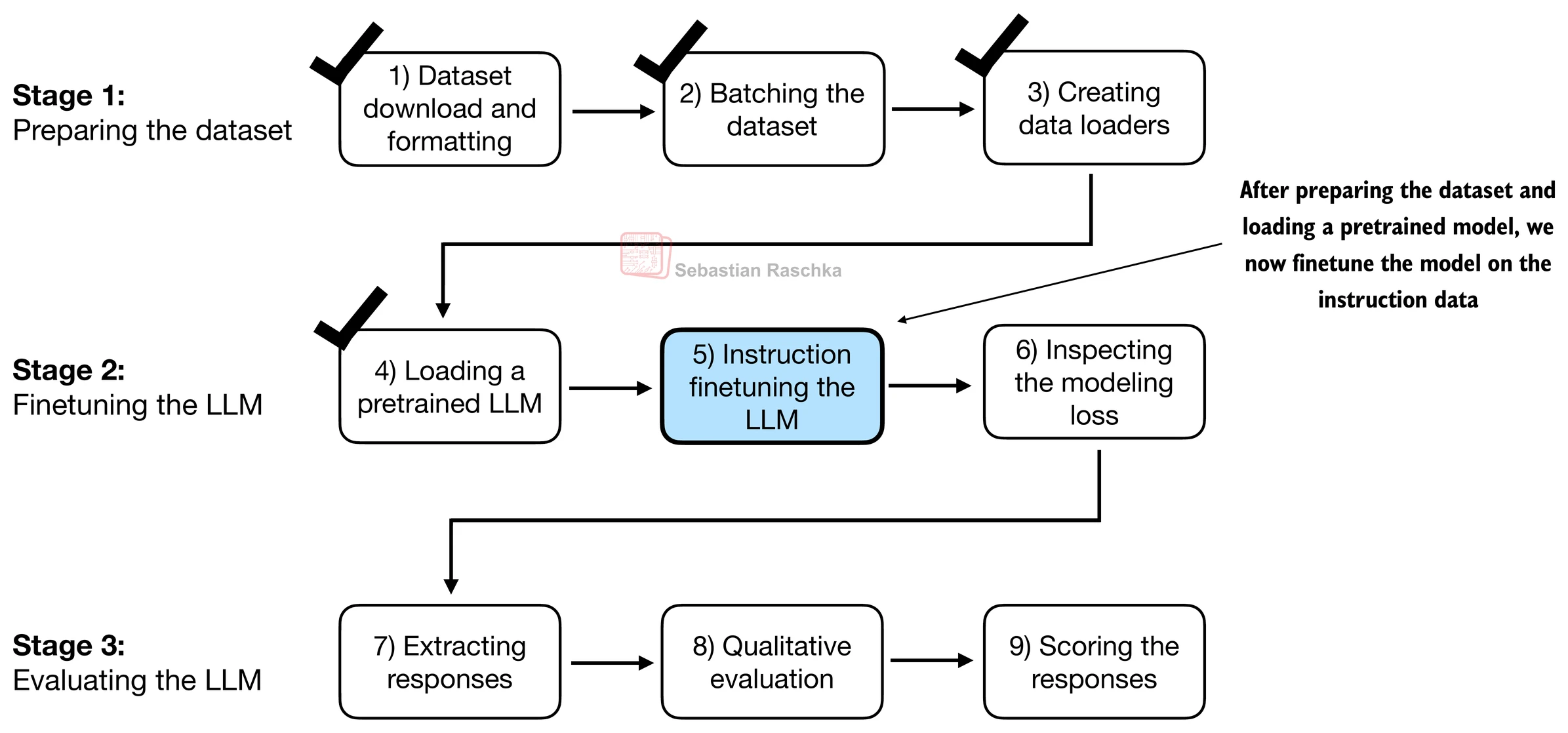
Note that we can reuse all the loss calculation and training functions that we used in previous chapters.

from previous_chapters import (
    calc_loss_loader,
    train_model_simple
)

Let’s calculate the initial training and validation set loss before we start training (as in previous chapters, the goal is to minimize the loss.)

model.to(device)

torch.manual_seed(123)

with torch.no_grad():
    train_loss = calc_loss_loader(train_loader, model, device, num_batches=5)
    val_loss = calc_loss_loader(val_loader, model, device, num_batches=5)

print("Training loss:", train_loss)
print("Validation loss:", val_loss)

Training loss: 3.82590913772583
Validation loss: 3.7619335651397705

The runtimes for various devices are shown for reference below (running this notebook on a compatible GPU device requires no changes to the code.)

Model	Device	Runtime for 2 Epochs
gpt2-medium (355M)	CPU (M3 MacBook Air)	15.78 minutes
gpt2-medium (355M)	GPU (M3 MacBook Air)	10.77 minutes
gpt2-medium (355M)	GPU (L4)	1.83 minutes
gpt2-medium (355M)	GPU (A100)	0.86 minutes
gpt2-small (124M)	CPU (M3 MacBook Air)	5.74 minutes
gpt2-small (124M)	GPU (M3 MacBook Air)	3.73 minutes
gpt2-small (124M)	GPU (L4)	0.69 minutes
gpt2-small (124M)	GPU (A100)	0.39 minutes

I ran this notebook using the "gpt2-medium (355M)" model on Google Colab.

import time

start_time = time.time()

torch.manual_seed(123)

optimizer = torch.optim.AdamW(model.parameters(), lr=0.00005, weight_decay=0.1)

num_epochs = 2

train_losses, val_losses, tokens_seen = train_model_simple(
    model, train_loader, val_loader, optimizer, device,
    num_epochs=num_epochs, eval_freq=5, eval_iter=5,
    start_context=format_input(val_data[0]), tokenizer=tokenizer
)

end_time = time.time()
execution_time_minutes = (end_time - start_time) / 60
print(f"Training completed in {execution_time_minutes:.2f} minutes.")

Ep 1 (Step 000000): Train loss 2.637, Val loss 2.626
Ep 1 (Step 000005): Train loss 1.174, Val loss 1.103
Ep 1 (Step 000010): Train loss 0.872, Val loss 0.944
Ep 1 (Step 000015): Train loss 0.857, Val loss 0.906
Ep 1 (Step 000020): Train loss 0.776, Val loss 0.881
Ep 1 (Step 000025): Train loss 0.754, Val loss 0.859
Ep 1 (Step 000030): Train loss 0.799, Val loss 0.836
Ep 1 (Step 000035): Train loss 0.714, Val loss 0.808
Ep 1 (Step 000040): Train loss 0.672, Val loss 0.806
Ep 1 (Step 000045): Train loss 0.633, Val loss 0.789
Ep 1 (Step 000050): Train loss 0.663, Val loss 0.783
Ep 1 (Step 000055): Train loss 0.760, Val loss 0.763
Ep 1 (Step 000060): Train loss 0.719, Val loss 0.743
Ep 1 (Step 000065): Train loss 0.653, Val loss 0.735
Ep 1 (Step 000070): Train loss 0.533, Val loss 0.729
Ep 1 (Step 000075): Train loss 0.568, Val loss 0.729
Ep 1 (Step 000080): Train loss 0.604, Val loss 0.725
Ep 1 (Step 000085): Train loss 0.509, Val loss 0.710
Ep 1 (Step 000090): Train loss 0.563, Val loss 0.691
Ep 1 (Step 000095): Train loss 0.502, Val loss 0.681
Ep 1 (Step 000100): Train loss 0.504, Val loss 0.677
Ep 1 (Step 000105): Train loss 0.565, Val loss 0.670
Ep 1 (Step 000110): Train loss 0.554, Val loss 0.666
Ep 1 (Step 000115): Train loss 0.508, Val loss 0.663
Below is an instruction that describes a task. Write a response that appropriately completes the request.  ### Instruction: Convert the active sentence to passive: 'The chef cooks the meal every day.'  ### Response: The meal is prepared every day by the chef.<|endoftext|>The following is an instruction that describes a task. Write a response that appropriately completes the request.  ### Instruction: Convert the active sentence to passive:
Ep 2 (Step 000120): Train loss 0.435, Val loss 0.671
Ep 2 (Step 000125): Train loss 0.451, Val loss 0.687
Ep 2 (Step 000130): Train loss 0.447, Val loss 0.682
Ep 2 (Step 000135): Train loss 0.405, Val loss 0.682
Ep 2 (Step 000140): Train loss 0.410, Val loss 0.681
Ep 2 (Step 000145): Train loss 0.369, Val loss 0.681
Ep 2 (Step 000150): Train loss 0.382, Val loss 0.675
Ep 2 (Step 000155): Train loss 0.414, Val loss 0.675
Ep 2 (Step 000160): Train loss 0.412, Val loss 0.684
Ep 2 (Step 000165): Train loss 0.379, Val loss 0.686
Ep 2 (Step 000170): Train loss 0.322, Val loss 0.680
Ep 2 (Step 000175): Train loss 0.338, Val loss 0.667
Ep 2 (Step 000180): Train loss 0.392, Val loss 0.656
Ep 2 (Step 000185): Train loss 0.415, Val loss 0.657
Ep 2 (Step 000190): Train loss 0.340, Val loss 0.647
Ep 2 (Step 000195): Train loss 0.328, Val loss 0.633
Ep 2 (Step 000200): Train loss 0.309, Val loss 0.633
Ep 2 (Step 000205): Train loss 0.353, Val loss 0.631
Ep 2 (Step 000210): Train loss 0.364, Val loss 0.630
Ep 2 (Step 000215): Train loss 0.394, Val loss 0.634
Ep 2 (Step 000220): Train loss 0.297, Val loss 0.644
Ep 2 (Step 000225): Train loss 0.342, Val loss 0.658
Ep 2 (Step 000230): Train loss 0.294, Val loss 0.656
Below is an instruction that describes a task. Write a response that appropriately completes the request.  ### Instruction: Convert the active sentence to passive: 'The chef cooks the meal every day.'  ### Response: The meal is cooked every day by the chef.<|endoftext|>The following is an instruction that describes a task. Write a response that appropriately completes the request.  ### Instruction: What is the capital of the United Kingdom
Training completed in 3.25 minutes.

As we can see based on the outputs above, the model trains well, as we can tell based on the decreasing training loss and validation loss values.

Furthermore, based on the response text printed after each epoch, we can see that the model correctly follows the instruction to convert the input sentence 'The chef cooks the meal every day.' into passive voice 'The meal is cooked every day by the chef.' (We will properly format and evaluate the responses in a later section)

Finally, let’s take a look at the training and validation loss curves

from previous_chapters import plot_losses

epochs_tensor = torch.linspace(0, num_epochs, len(train_losses))
plot_losses(epochs_tensor, tokens_seen, train_losses, val_losses)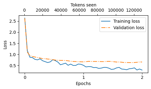

As we can see, the loss decreases sharply at the beginning of the first epoch, which means the model starts learning quickly. We can see that slight overfitting sets in at around 1 training epoch.

Stage 3: Evaluating LLM¶

Extract and save responses¶

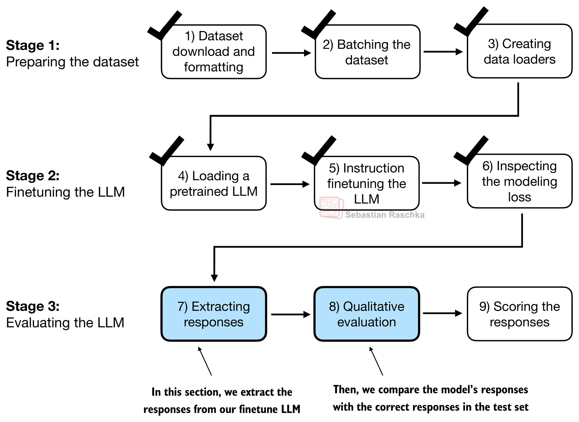
We save the test set responses for scoring in the next section
We also save a copy of the model for future use

But first, let’s take a brief look at the responses generated by the finetuned model.

torch.manual_seed(123)


for entry in test_data[:3]:

    input_text = format_input(entry)

    token_ids = generate(
        model=model,
        idx=text_to_token_ids(input_text, tokenizer).to(device),
        max_new_tokens=256,
        context_size=BASE_CONFIG["context_length"],
        eos_id=50256
    )
    generated_text = token_ids_to_text(token_ids, tokenizer)
    response_text = (
        generated_text[len(input_text):]
        .replace("### Response:", "")
        .strip()
)

    print(input_text)
    print(f"\nCorrect response:\n>> {entry['output']}")
    print(f"\nModel response:\n>> {response_text.strip()}")
    print("-------------------------------------")

Below is an instruction that describes a task. Write a response that appropriately completes the request.

### Instruction:
Rewrite the sentence using a simile.

### Input:
The car is very fast.

Correct response:
>> The car is as fast as lightning.

Model response:
>> The car is as fast as a bullet.
-------------------------------------
Below is an instruction that describes a task. Write a response that appropriately completes the request.

### Instruction:
What type of cloud is typically associated with thunderstorms?

Correct response:
>> The type of cloud typically associated with thunderstorms is cumulonimbus.

Model response:
>> The type of cloud associated with thunderstorms is a cumulus cloud.
-------------------------------------
Below is an instruction that describes a task. Write a response that appropriately completes the request.

### Instruction:
Name the author of 'Pride and Prejudice'.

Correct response:
>> Jane Austen.

Model response:
>> The author of 'Pride and Prejudice' is Jane Austen.
-------------------------------------

As we can see based on the test set instructions, given responses, and the model’s responses, the model performs relatively well
The answers to the first and last instructions are clearly correct
The second answer is close; the model answers with “cumulus cloud” instead of “cumulonimbus” (however, note that cumulus clouds can develop into cumulonimbus clouds, which are capable of producing thunderstorms)
Most importantly, we can see that model evaluation is not as straightforward as in the previous chapter, where we just had to calculate the percentage of correct spam/non-spam class labels to obtain the classification accuracy.
In practice, instruction-finetuned LLMs such as chatbots are evaluated via multiple approaches:
- short-answer and multiple choice benchmarks such as MMLU (“Measuring Massive Multitask Language Understanding”, https://arxiv.org/abs/2009.03300), which test the knowledge of a model
- human preference comparison to other LLMs, such as LMSYS chatbot arena (https://arena.lmsys.org)
- automated conversational benchmarks, where another LLM like GPT-4 is used to evaluate the responses, such as AlpacaEval (https://tatsu-lab.github.io/alpaca_eval/)

In the next section, we will use an approach similar to AlpacaEval and use another LLM to evaluate the responses of our model; however, we will use our own test set instead of using a publicly available benchmark dataset.

For this, we add the model response to the test_data dictionary and save it as a "instruction-data-with-response.json" file for record-keeping so that we can load and analyze it in separate Python sessions if needed.

from tqdm import tqdm

for i, entry in tqdm(enumerate(test_data), total=len(test_data)):

    input_text = format_input(entry)

    token_ids = generate(
        model=model,
        idx=text_to_token_ids(input_text, tokenizer).to(device),
        max_new_tokens=256,
        context_size=BASE_CONFIG["context_length"],
        eos_id=50256
    )
    generated_text = token_ids_to_text(token_ids, tokenizer)
    response_text = generated_text[len(input_text):].replace("### Response:", "").strip()

    test_data[i]["model_response"] = response_text


with open("instruction-data-with-response.json", "w") as file:
    json.dump(test_data, file, indent=4)  # "indent" for pretty-printing

100%|██████████| 110/110 [01:09<00:00,  1.59it/s]

Let’s double-check one of the entries to see whether the responses have been added to the test_data dictionary correctly.

print(test_data[0])

{'instruction': 'Rewrite the sentence using a simile.', 'input': 'The car is very fast.', 'output': 'The car is as fast as lightning.', 'model_response': 'The car is as fast as a bullet.'}

Finally, we also save the model in case we want to reuse it in the future.

import re


file_name = f"{re.sub(r'[ ()]', '', CHOOSE_MODEL) }-sft.pth"
torch.save(model.state_dict(), file_name)
print(f"Model saved as {file_name}")

Model saved as gpt2-medium355M-sft.pth

Evaluating the finetuned LLM¶

DISCLAIMER: Don’t execute the following code, read only.

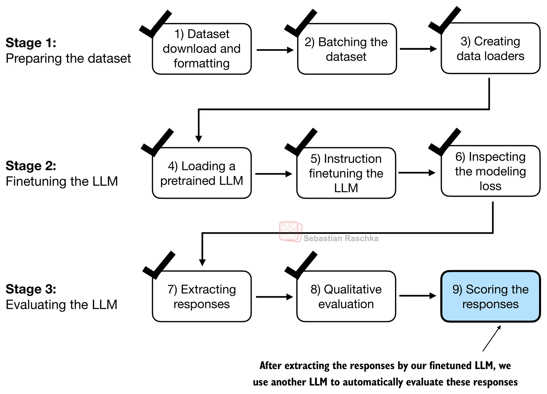
We automate the response evaluation of the finetuned LLM using another, larger LLM

In particular, we use an instruction-finetuned 8-billion-parameter Llama 3 model by Meta AI that can be run locally via ollama (https://ollama.com).
- Ollama is an application to run LLMs efficiently
- It is a wrapper around llama.cpp (https://github.com/ggerganov/llama.cpp), which implements LLMs in pure C/C++ to maximize efficiency
- Note that it is a tool for using LLMs to generate text (inference), not training or finetuning LLMs
- Before running the code below, install ollama by visiting https://ollama.com and following the instructions (for instance, clicking on the “Download” button and downloading the ollama application for your operating system)

For macOS and Windows users, click on the ollama application you downloaded; if it prompts you to install the command line usage, say “yes”
Linux users can use the installation command provided on the ollama website
In general, before we can use ollama from the command line, we have to either start the ollama application or run ollama serve in a separate terminal

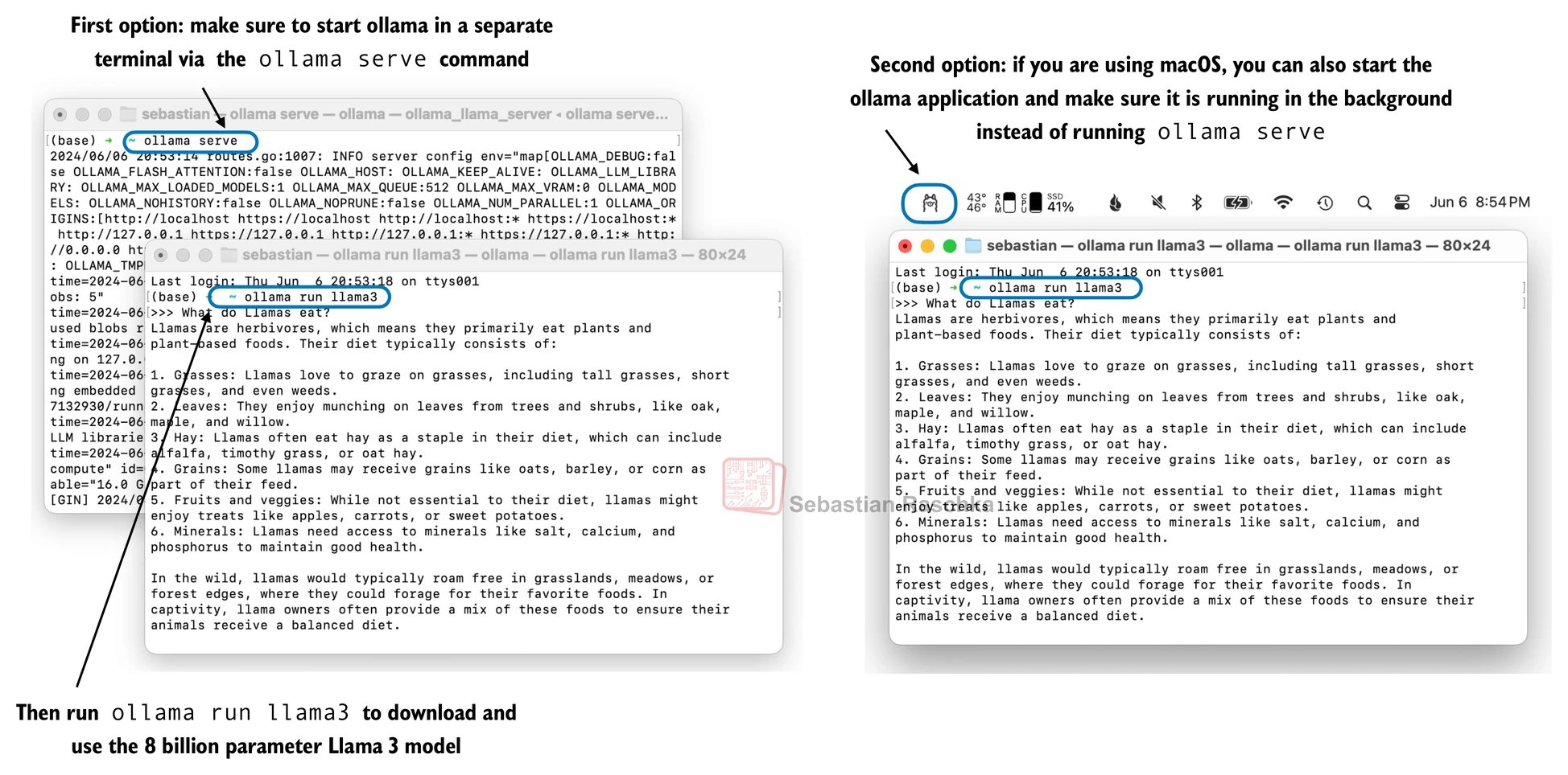
Note:

When running ollama serve in the terminal, as described above, you may encounter an error message saying Error: listen tcp 127.0.0.1:11434: bind: address already in use
If that’s the case, try use the command OLLAMA_HOST=127.0.0.1:11435 ollama serve (and if this address is also in use, try to increment the numbers by one until you find an address not in use

With the ollama application or ollama serve running in a different terminal, on the command line, execute the following command to try out the 8-billion-parameter Llama 3 model (the model, which takes up 4.7 GB of storage space, will be automatically downloaded the first time you execute this command)

# 8B model
ollama run llama3

The output looks like as follows

$ ollama run llama3
pulling manifest
pulling 6a0746a1ec1a... 100% ▕████████████████▏ 4.7 GB
pulling 4fa551d4f938... 100% ▕████████████████▏  12 KB
pulling 8ab4849b038c... 100% ▕████████████████▏  254 B
pulling 577073ffcc6c... 100% ▕████████████████▏  110 B
pulling 3f8eb4da87fa... 100% ▕████████████████▏  485 B
verifying sha256 digest
writing manifest
removing any unused layers
success

Note that llama3 refers to the instruction finetuned 8-billion-parameter Llama 3 model
Using ollama with the "llama3" model (a 8B parameter model) requires 16 GB of RAM; if this is not supported by your machine, you can try the smaller model, such as the 3.8B parameter phi-3 model by setting model = "phi-3", which only requires 8 GB of RAM
Alternatively, you can also use the larger 70-billion-parameter Llama 3 model, if your machine supports it, by replacing llama3 with llama3:70b
After the download has been completed, you will see a command line prompt that allows you to chat with the model
Try a prompt like “What do llamas eat?”, which should return an output similar to the following

>>> What do llamas eat?
Llamas are ruminant animals, which means they have a four-chambered
stomach and eat plants that are high in fiber. In the wild, llamas
typically feed on:
1. Grasses: They love to graze on various types of grasses, including tall
grasses, wheat, oats, and barley.

You can end this session using the input /bye

The following code checks whether the ollama session is running correctly before proceeding to use ollama to evaluate the test set responses we generated in the previous section

import psutil

def check_if_running(process_name):
    running = False
    for proc in psutil.process_iter(["name"]):
        if process_name in proc.info["name"]:
            running = True
            break
    return running

ollama_running = check_if_running("ollama")

if not ollama_running:
    raise RuntimeError("Ollama not running. Launch ollama before proceeding.")
print("Ollama running:", check_if_running("ollama"))

Ollama running: True

# This cell is optional; it allows you to restart the notebook
# and only run section 7.7 without rerunning any of the previous code
import json
from tqdm import tqdm

file_path = "instruction-data-with-response.json"

with open(file_path, "r") as file:
    test_data = json.load(file)


def format_input(entry):
    instruction_text = (
        f"Below is an instruction that describes a task. "
        f"Write a response that appropriately completes the request."
        f"\n\n### Instruction:\n{entry['instruction']}"
    )

    input_text = f"\n\n### Input:\n{entry['input']}" if entry["input"] else ""

    return instruction_text + input_text

Now, an alternative way to the ollama run command we used earlier to interact with the model is via its REST API in Python via the following function
Before you run the next cells in this notebook, make sure that ollama is still running (the previous code cells should print "Ollama running: True")
Next, run the following code cell to query the model

import requests  # noqa: F811
# import urllib.request

def query_model(
    prompt,
    model="llama3",
    # If you used OLLAMA_HOST=127.0.0.1:11435 ollama serve
    # update the address from 11434 to 11435
    url="https://courses.brianjalaian.com/api/chat"
):
    # Create the data payload as a dictionary
    data = {
        "model": model,
        "messages": [
            {"role": "user", "content": prompt}
        ],
        "options": {     # Settings below are required for deterministic responses
            "seed": 123,
            "temperature": 0,
            "num_ctx": 2048
        }
    }


    """
    # Convert the dictionary to a JSON formatted string and encode it to bytes
    payload = json.dumps(data).encode("utf-8")

    # Create a request object, setting the method to POST and adding necessary headers
    request = urllib.request.Request(
        url,
        data=payload,
        method="POST"
    )
    request.add_header("Content-Type", "application/json")

    # Send the request and capture the response
    response_data = ""
    with urllib.request.urlopen(request) as response:
        # Read and decode the response
        while True:
            line = response.readline().decode("utf-8")
            if not line:
                break
            response_json = json.loads(line)
            response_data += response_json["message"]["content"]

    return response_data
    """

    # The book originally used the commented-out above, which is based
    # on urllib. It works generally fine, but some readers reported
    # issues with using urlib when using a (company) VPN.
    # The code below uses the requests library, which doesn't seem
    # to have these issues.

    # Send the POST request
    with requests.post(url, json=data, stream=True, timeout=30) as r:
        r.raise_for_status()
        response_data = ""
        for line in r.iter_lines(decode_unicode=True):
            if not line:
                continue
            response_json = json.loads(line)
            if "message" in response_json:
                response_data += response_json["message"]["content"]

    return response_data


model = "llama3"
result = query_model("What do Llamas eat?", model)
print(result)

Llamas are herbivores, which means they primarily feed on plant-based foods. Their diet typically consists of:

1. Grasses: Llamas love to graze on various types of grasses, including tall grasses, short grasses, and even weeds.
2. Hay: High-quality hay, such as alfalfa or timothy hay, is a staple in a llama's diet. They enjoy the sweet taste and texture of fresh hay.
3. Grains: Llamas may receive grains like oats, barley, or corn as part of their daily ration. However, it's essential to provide these grains in moderation, as they can be high in calories.
4. Fruits and vegetables: Llamas enjoy a variety of fruits and veggies, such as apples, carrots, sweet potatoes, and leafy greens like kale or spinach.
5. Minerals: Llamas require access to mineral supplements, which help maintain their overall health and well-being.

In the wild, llamas might also eat:

1. Leaves: They'll munch on leaves from trees and shrubs, including plants like willow, alder, and birch.
2. Bark: In some cases, llamas may eat the bark of certain trees, like aspen or cottonwood.
3. Mosses and lichens: These non-vascular plants can be a tasty snack for llamas.

In captivity, llama owners typically provide a balanced diet that includes a mix of hay, grains, and fruits/vegetables. It's essential to consult with a veterinarian or experienced llama breeder to determine the best feeding plan for your llama.

Note that if you are getting an HTTPError: 404 Client Error: Not Found for url: https://courses.brianjalaian.com/api/chat error, this could mean you haven’t downloaded the llama3 model yet (to download the model, either use the UI or ollama run llama3 on the terminal)

Now, using the query_model function we defined above, we can evaluate the responses of our finetuned model; let’s try it out on the first 3 test set responses we looked at in a previous section

for entry in test_data[:3]:
    prompt = (
        f"Given the input `{format_input(entry)}` "
        f"and correct output `{entry['output']}`, "
        f"score the model response `{entry['model_response']}`"
        f" on a scale from 0 to 100, where 100 is the best score. "
    )
    print("\nDataset response:")
    print(">>", entry['output'])
    print("\nModel response:")
    print(">>", entry["model_response"])
    print("\nScore:")
    print(">>", query_model(prompt))
    print("\n-------------------------")


Dataset response:
>> The car is as fast as lightning.

Model response:
>> The car is as fast as a bullet.

Score:
>> I'd rate the model response "The car is as fast as a bullet." an 85 out of 100.

Here's why:

* The response uses a simile correctly, comparing the speed of the car to something else (in this case, a bullet).
* The comparison is relevant and makes sense, as bullets are known for their high velocity.
* The phrase "as fast as" is used correctly to introduce the simile.

The only reason I wouldn't give it a perfect score is that some people might find the comparison slightly less vivid or evocative than others. For example, comparing something to lightning (as in the original response) can be more dramatic and attention-grabbing. However, "as fast as a bullet" is still a strong and effective simile that effectively conveys the idea of the car's speed.

Overall, I think the model did a great job!

-------------------------

Dataset response:
>> The type of cloud typically associated with thunderstorms is cumulonimbus.

Model response:
>> The type of cloud associated with thunderstorms is a cumulus cloud.

Score:
>> I'd score this model response as 40 out of 100.

Here's why:

* The model correctly identifies that thunderstorms are related to clouds (correctly identifying the type of phenomenon).
* However, it incorrectly specifies the type of cloud associated with thunderstorms. Cumulus clouds are not typically associated with thunderstorms; cumulonimbus clouds are.
* The response lacks precision and accuracy in its description.

Overall, while the model attempts to address the instruction, it provides an incorrect answer, which is a significant error.

-------------------------

Dataset response:
>> Jane Austen.

Model response:
>> The author of 'Pride and Prejudice' is Jane Austen.

Score:
>> I'd rate my own response as 95 out of 100. Here's why:

* The response accurately answers the question by naming the author of 'Pride and Prejudice' as Jane Austen.
* The response is concise and clear, making it easy to understand.
* There are no grammatical errors or ambiguities that could lead to confusion.

The only reason I wouldn't give myself a perfect score is that the response is slightly redundant - it's not necessary to rephrase the question in the answer. A more concise response would be simply "Jane Austen."

-------------------------

Note: Better evaluation prompt

A reader (Ayoosh Kathuria) suggested a longer, improved prompt that evaluates responses on a scale of 1–5 (instead of 1 to 100) and employs a grading rubric, resulting in more accurate and less noisy evaluations:

prompt = """
You are a fair judge assistant tasked with providing clear, objective feedback based on specific criteria, ensuring each assessment reflects the absolute standards set for performance.
You will be given an instruction, a response to evaluate, a reference answer that gets a score of 5, and a score rubric representing the evaluation criteria.
Write a detailed feedback that assess the quality of the response strictly based on the given score rubric, not evaluating in general.
Please do not generate any other opening, closing, and explanations.

Here is the rubric you should use to build your answer:
1: The response fails to address the instructions, providing irrelevant, incorrect, or excessively verbose information that detracts from the user's request.
2: The response partially addresses the instructions but includes significant inaccuracies, irrelevant details, or excessive elaboration that detracts from the main task.
3: The response follows the instructions with some minor inaccuracies or omissions. It is generally relevant and clear, but may include some unnecessary details or could be more concise.
4: The response adheres to the instructions, offering clear, accurate, and relevant information in a concise manner, with only occasional, minor instances of excessive detail or slight lack of clarity.
5: The response fully adheres to the instructions, providing a clear, accurate, and relevant answer in a concise and efficient manner. It addresses all aspects of the request without unnecessary details or elaboration

Provide your feedback as follows:

Feedback:::
Evaluation: (your rationale for the rating, as a text)
Total rating: (your rating, as a number between 1 and 5)

You MUST provide values for 'Evaluation:' and 'Total rating:' in your answer.

Now here is the instruction, the reference answer, and the response.

Instruction: {instruction}
Reference Answer: {reference}
Answer: {answer}


Provide your feedback. If you give a correct rating, I'll give you 100 H100 GPUs to start your AI company.
Feedback:::
Evaluation: """

For more context and information, see this GitHub discussion

As we can see, the Llama 3 model provides a reasonable evaluation and also gives partial points if a model is not entirely correct, as we can see based on the “cumulus cloud” answer
Note that the previous prompt returns very verbose evaluations; we can tweak the prompt to generate integer responses in the range between 0 and 100 (where 100 is best) to calculate an average score for our model
The evaluation of the 110 entries in the test set takes about 1 minute on an M3 MacBook Air laptop

def generate_model_scores(json_data, json_key, model="llama3"):
    scores = []
    for entry in tqdm(json_data, desc="Scoring entries"):
        prompt = (
            f"Given the input `{format_input(entry)}` "
            f"and correct output `{entry['output']}`, "
            f"score the model response `{entry[json_key]}`"
            f" on a scale from 0 to 100, where 100 is the best score. "
            f"Respond with the integer number only."
        )
        score = query_model(prompt, model)
        try:
            scores.append(int(score))
        except ValueError:
            print(f"Could not convert score: {score}")
            continue

    return scores


scores = generate_model_scores(test_data, "model_response")
print(f"Number of scores: {len(scores)} of {len(test_data)}")
print(f"Average score: {sum(scores)/len(scores):.2f}\n")

Scoring entries: 100%|████████████████████████| 110/110 [00:37<00:00,  2.90it/s]

Number of scores: 110 of 110
Average score: 49.45

Our model achieves an average score of above 50, which we can use as a reference point to compare the model to other models or to try out other training settings that may improve the model
Note that ollama is not fully deterministic across operating systems (as of this writing), so the numbers you are getting might slightly differ from the ones shown above

For reference, the original
- Llama 3 8B base model achieves a score of 58.51
- Llama 3 8B instruct model achieves a score of 82.65