Creator: Chung-En Johnny Yu
Content updated: 2026-02-20
Source:
Build a Large Language Model From Scratch by Sebastian Raschka - Ch6
Hands-on practice this notebook on your Google Colab:
Now, run the code and practice it!
Additional resources:
To be added.
from importlib.metadata import version

pkgs = ["matplotlib",  # Plotting library
        "numpy",       # PyTorch & TensorFlow dependency
        "tiktoken",    # Tokenizer
        "torch",       # Deep learning library
        "tensorflow",  # For OpenAI's pretrained weights
        "pandas"       # Dataset loading
       ]
for p in pkgs:
    print(f"{p} version: {version(p)}")
matplotlib version: 3.10.0
numpy version: 2.0.2
tiktoken version: 0.12.0
torch version: 2.10.0+cu128
tensorflow version: 2.19.0
pandas version: 2.2.2
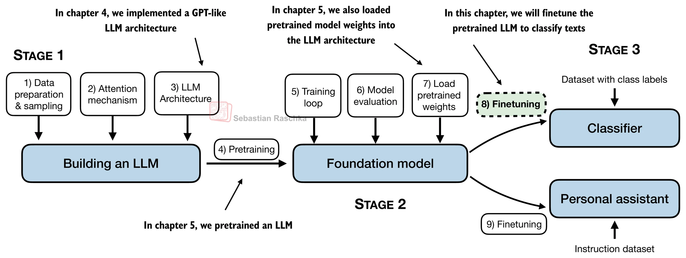
Categories of finetuning
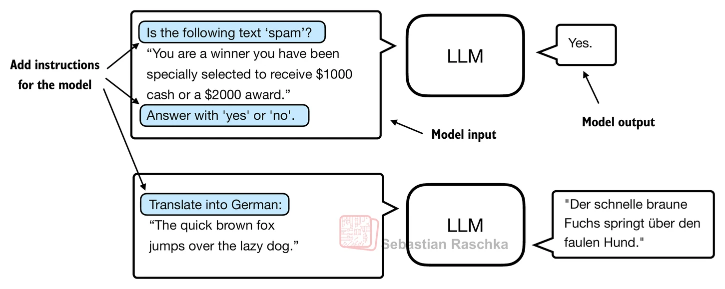
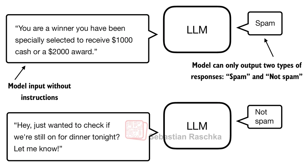
It’s similar to training a convolutional network to classify handwritten digits. In classification finetuning, we have a specific number of class labels (for example, “spam” and “not spam”) that the model can output. A classification finetuned model can only predict classes it has seen during training (for example, “spam” or “not spam”), whereas an instruction-finetuned model can usually perform many tasks. We can think of a classification-finetuned model as a very specialized model; in practice, it is much easier to create a specialized model than a generalist model that performs well on many different tasks.
The following steps are similar to what we do in machine learning.
Preparing the dataset
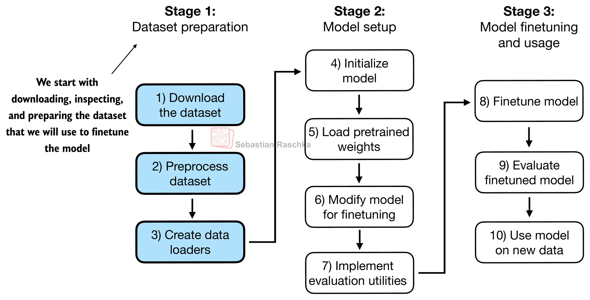
We use a dataset consisting of spam and non-spam text messages to finetune the LLM to classify them.
import requests
import zipfile
import os
from pathlib import Path

url = "https://archive.ics.uci.edu/static/public/228/sms+spam+collection.zip"
zip_path = "sms_spam_collection.zip"
extracted_path = "sms_spam_collection"
data_file_path = Path(extracted_path) / "SMSSpamCollection.tsv"


def download_and_unzip_spam_data(url, zip_path, extracted_path, data_file_path):
    if data_file_path.exists():
        print(f"{data_file_path} already exists. Skipping download and extraction.")
        return

    # Downloading the file
    response = requests.get(url, stream=True, timeout=60)
    response.raise_for_status()
    with open(zip_path, "wb") as out_file:
        for chunk in response.iter_content(chunk_size=8192):
            if chunk:
                out_file.write(chunk)

    # Unzipping the file
    with zipfile.ZipFile(zip_path, "r") as zip_ref:
        zip_ref.extractall(extracted_path)

    # Add .tsv file extension
    original_file_path = Path(extracted_path) / "SMSSpamCollection"
    os.rename(original_file_path, data_file_path)
    print(f"File downloaded and saved as {data_file_path}")


try:
    download_and_unzip_spam_data(url, zip_path, extracted_path, data_file_path)
except (requests.exceptions.RequestException, TimeoutError) as e:
    print(f"Primary URL failed: {e}. Trying backup URL...")
    url = "https://f001.backblazeb2.com/file/LLMs-from-scratch/sms%2Bspam%2Bcollection.zip"
    download_and_unzip_spam_data(url, zip_path, extracted_path, data_file_path)


# The book originally used the following code below
# However, urllib uses older protocol settings that
# can cause problems for some readers using a VPN.
# The `requests` version above is more robust
# in that regard.

"""
import urllib.request
import zipfile
import os
from pathlib import Path

url = "https://archive.ics.uci.edu/static/public/228/sms+spam+collection.zip"
zip_path = "sms_spam_collection.zip"
extracted_path = "sms_spam_collection"
data_file_path = Path(extracted_path) / "SMSSpamCollection.tsv"

def download_and_unzip_spam_data(url, zip_path, extracted_path, data_file_path):
    if data_file_path.exists():
        print(f"{data_file_path} already exists. Skipping download and extraction.")
        return

    # Downloading the file
    with urllib.request.urlopen(url) as response:
        with open(zip_path, "wb") as out_file:
            out_file.write(response.read())

    # Unzipping the file
    with zipfile.ZipFile(zip_path, "r") as zip_ref:
        zip_ref.extractall(extracted_path)

    # Add .tsv file extension
    original_file_path = Path(extracted_path) / "SMSSpamCollection"
    os.rename(original_file_path, data_file_path)
    print(f"File downloaded and saved as {data_file_path}")

try:
    download_and_unzip_spam_data(url, zip_path, extracted_path, data_file_path)
except (urllib.error.HTTPError, urllib.error.URLError, TimeoutError) as e:
    print(f"Primary URL failed: {e}. Trying backup URL...")
    url = "https://f001.backblazeb2.com/file/LLMs-from-scratch/sms%2Bspam%2Bcollection.zip"
    download_and_unzip_spam_data(url, zip_path, extracted_path, data_file_path)
"""
sms_spam_collection/SMSSpamCollection.tsv already exists. Skipping download and extraction.
The dataset is saved as a tab-separated text file, which we can load into a pandas DataFrame.
import pandas as pd

df = pd.read_csv(data_file_path, sep="\t", header=None, names=["Label", "Text"])
dfWhen we check the class distribution, we see that the data contains “ham” (i.e., “not spam”) much more frequently than “spam”.
print(df["Label"].value_counts())Label
ham 4825
spam 747
Name: count, dtype: int64
For simplicity, and because we prefer a small dataset for educational purposes anyway (it will make it possible to finetune the LLM faster), we subsample (undersample) the dataset so that it contains 747 instances from each class.
def create_balanced_dataset(df):

    # Count the instances of "spam"
    num_spam = df[df["Label"] == "spam"].shape[0]

    # Randomly sample "ham" instances to match the number of "spam" instances
    ham_subset = df[df["Label"] == "ham"].sample(num_spam, random_state=123)

    # Combine ham "subset" with "spam"
    balanced_df = pd.concat([ham_subset, df[df["Label"] == "spam"]])

    return balanced_df


balanced_df = create_balanced_dataset(df)
print(balanced_df["Label"].value_counts())
Label
ham 747
spam 747
Name: count, dtype: int64
Next, we change the string class labels “ham” and “spam” into integer class labels 0 and 1:
balanced_df["Label"] = balanced_df["Label"].map({"ham": 0, "spam": 1})balanced_dfLet’s now define a function that randomly divides the dataset into training, validation, and test subsets.
def random_split(df, train_frac, validation_frac):
    # Shuffle the entire DataFrame
    df = df.sample(frac=1, random_state=123).reset_index(drop=True)

    # Calculate split indices
    train_end = int(len(df) * train_frac)
    validation_end = train_end + int(len(df) * validation_frac)

    # Split the DataFrame
    train_df = df[:train_end]
    validation_df = df[train_end:validation_end]
    test_df = df[validation_end:]

    return train_df, validation_df, test_df

train_df, validation_df, test_df = random_split(balanced_df, 0.7, 0.1)
# Test size is implied to be 0.2 as the remainder

train_df.to_csv("train.csv", index=None)
validation_df.to_csv("validation.csv", index=None)
test_df.to_csv("test.csv", index=None)
Creating data loaders
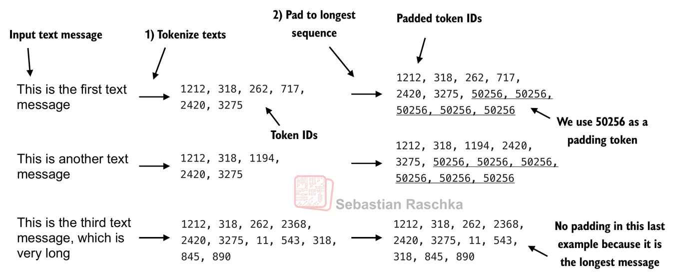
Note that the text messages have different lengths; if we want to combine multiple training examples in a batch, we have to either:
Truncate all messages to the length of the shortest message in the dataset or batch.
Pad all messages to the length of the longest message in the dataset or batch.
We choose option 2 and pad all messages to the longest message in the dataset with <|endoftext|> as a padding token.
import tiktoken

tokenizer = tiktoken.get_encoding("gpt2")
print(tokenizer.encode("<|endoftext|>", allowed_special={"<|endoftext|>"}))
[50256]
The SpamDataset class below identifies the longest sequence in the training dataset and adds the padding token to the others to match that sequence length:
import torch
from torch.utils.data import Dataset


class SpamDataset(Dataset):
    def __init__(self, csv_file, tokenizer, max_length=None, pad_token_id=50256):
        self.data = pd.read_csv(csv_file)

        # Pre-tokenize texts
        self.encoded_texts = [
            tokenizer.encode(text) for text in self.data["Text"]
        ]

        if max_length is None:
            self.max_length = self._longest_encoded_length()
        else:
            self.max_length = max_length
            # Truncate sequences if they are longer than max_length
            self.encoded_texts = [
                encoded_text[:self.max_length]
                for encoded_text in self.encoded_texts
            ]

        # Pad sequences to the longest sequence
        self.encoded_texts = [
            encoded_text + [pad_token_id] * (self.max_length - len(encoded_text))
            for encoded_text in self.encoded_texts
        ]

    def __getitem__(self, index):
        encoded = self.encoded_texts[index]
        label = self.data.iloc[index]["Label"]
        return (
            torch.tensor(encoded, dtype=torch.long),
            torch.tensor(label, dtype=torch.long)
        )

    def __len__(self):
        return len(self.data)

    def _longest_encoded_length(self):
        max_length = 0
        for encoded_text in self.encoded_texts:
            encoded_length = len(encoded_text)
            if encoded_length > max_length:
                max_length = encoded_length
        return max_length
train_dataset = SpamDataset(
csv_file="train.csv",
max_length=None,
tokenizer=tokenizer
)
print(train_dataset.max_length)120
We also pad the validation and test set to the longest training sequence.
Note that validation and test set samples that are longer than the longest training example are being truncated via
encoded_text[:self.max_length]in theSpamDatasetcode.This behavior is entirely optional, and it would also work well if we set
max_length=Nonein both the validation and test set cases.
val_dataset = SpamDataset(
    csv_file="validation.csv",
    max_length=train_dataset.max_length,
    tokenizer=tokenizer
)
test_dataset = SpamDataset(
    csv_file="test.csv",
    max_length=train_dataset.max_length,
    tokenizer=tokenizer
)
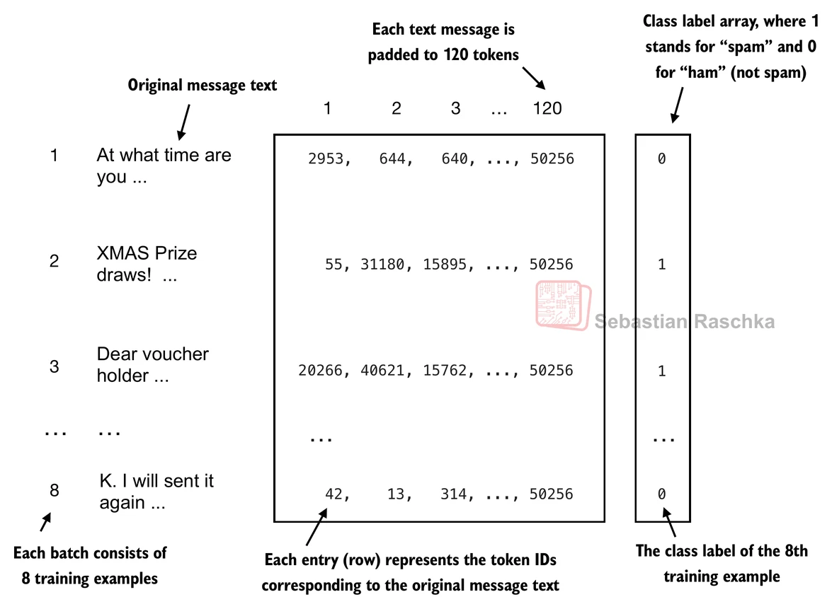
Next, we use the dataset to instantiate the data loaders.
from torch.utils.data import DataLoader

num_workers = 0
batch_size = 8

torch.manual_seed(123)

train_loader = DataLoader(
    dataset=train_dataset,
    batch_size=batch_size,
    shuffle=True,
    num_workers=num_workers,
    drop_last=True,
)

val_loader = DataLoader(
    dataset=val_dataset,
    batch_size=batch_size,
    num_workers=num_workers,
    drop_last=False,
)

test_loader = DataLoader(
    dataset=test_dataset,
    batch_size=batch_size,
    num_workers=num_workers,
    drop_last=False,
)
As a verification step, we iterate through the data loaders and ensure that the batches contain 8 training examples each, where each training example consists of 120 tokens.
print("Train loader:")
for input_batch, target_batch in train_loader:
    pass

print("Input batch dimensions:", input_batch.shape)
print("Label batch dimensions", target_batch.shape)
Train loader:
Input batch dimensions: torch.Size([8, 120])
Label batch dimensions torch.Size([8])
Lastly, let’s print the total number of batches in each dataset.
print(f"{len(train_loader)} training batches")
print(f"{len(val_loader)} validation batches")
print(f"{len(test_loader)} test batches")
130 training batches
19 validation batches
38 test batches
Initializing model with pretrained weights
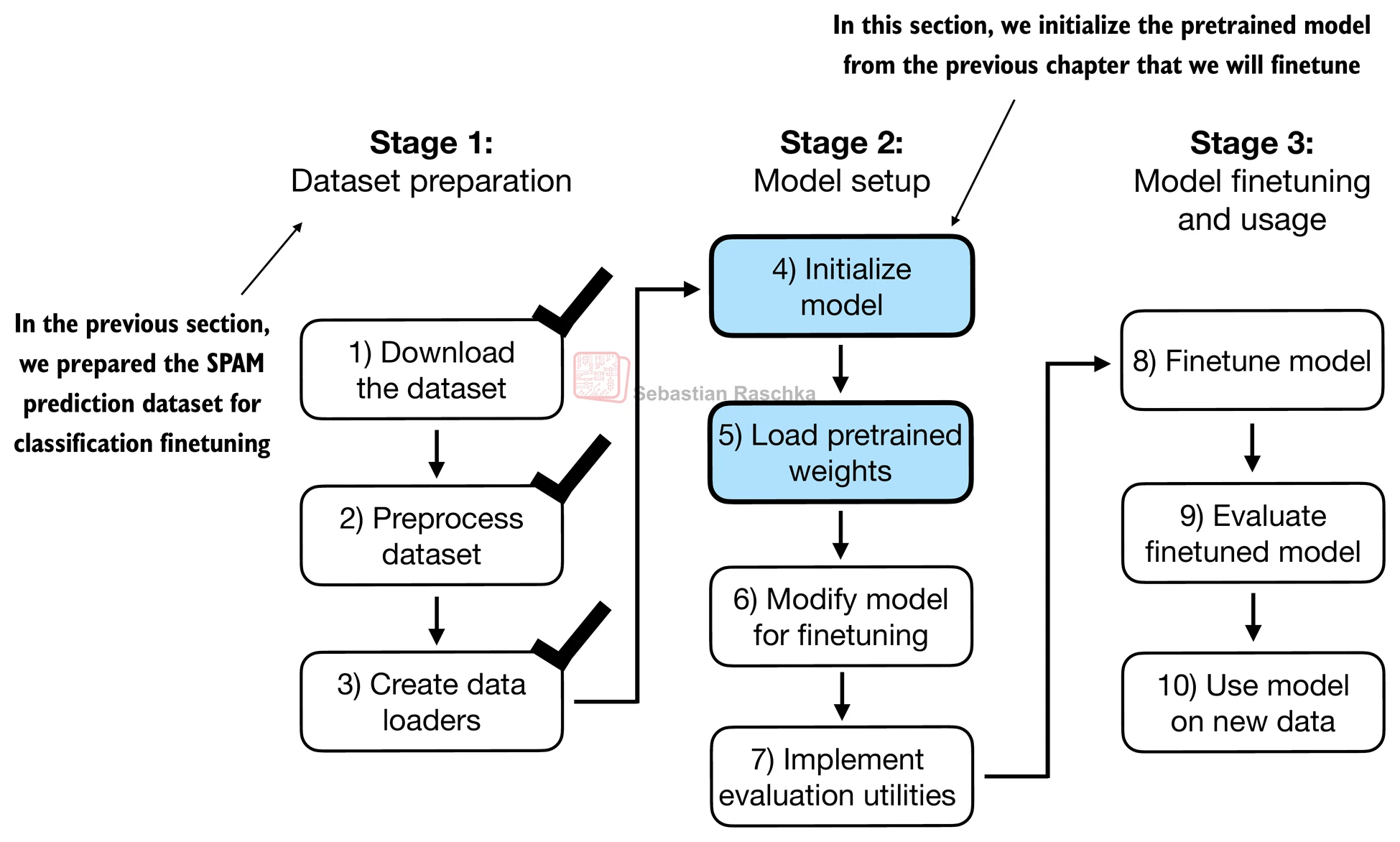
We initialize the pretrained model we worked with in the previous chapter.
CHOOSE_MODEL = "gpt2-small (124M)"
INPUT_PROMPT = "Every effort moves"

BASE_CONFIG = {
    "vocab_size": 50257,     # Vocabulary size
    "context_length": 1024,  # Context length
    "drop_rate": 0.0,        # Dropout rate
    "qkv_bias": True         # Query-key-value bias
}

model_configs = {
    "gpt2-small (124M)": {"emb_dim": 768, "n_layers": 12, "n_heads": 12},
    "gpt2-medium (355M)": {"emb_dim": 1024, "n_layers": 24, "n_heads": 16},
    "gpt2-large (774M)": {"emb_dim": 1280, "n_layers": 36, "n_heads": 20},
    "gpt2-xl (1558M)": {"emb_dim": 1600, "n_layers": 48, "n_heads": 25},
}

BASE_CONFIG.update(model_configs[CHOOSE_MODEL])

assert train_dataset.max_length <= BASE_CONFIG["context_length"], (
    f"Dataset length {train_dataset.max_length} exceeds model's context "
    f"length {BASE_CONFIG['context_length']}. Reinitialize data sets with "
    f"`max_length={BASE_CONFIG['context_length']}`"
)
# Download the file from my github
# Note that we save the file in the temporary folder of Google Colab,
# it will dispear once you close the session.
!wget -O /content/previous_chapters.py https://raw.githubusercontent.com/brianjalaian/CAP6606_ML_ISR/main/modules/02-LLM/05-finetuning_classification/data/previous_chapters.py
!wget -O /content/gpt_download.py https://raw.githubusercontent.com/brianjalaian/CAP6606_ML_ISR/main/modules/02-LLM/05-finetuning_classification/data/gpt_download.pyfrom gpt_download import download_and_load_gpt2
from previous_chapters import GPTModel, load_weights_into_gpt
model_size = CHOOSE_MODEL.split(" ")[-1].lstrip("(").rstrip(")")
settings, params = download_and_load_gpt2(model_size=model_size, models_dir="gpt2")
model = GPTModel(BASE_CONFIG)
load_weights_into_gpt(model, params)
model.eval();checkpoint: 100%|██████████| 77.0/77.0 [00:00<00:00, 130kiB/s]
encoder.json: 100%|██████████| 1.04M/1.04M [00:00<00:00, 3.03MiB/s]
hparams.json: 100%|██████████| 90.0/90.0 [00:00<00:00, 190kiB/s]
model.ckpt.data-00000-of-00001: 100%|██████████| 498M/498M [00:32<00:00, 15.4MiB/s]
model.ckpt.index: 100%|██████████| 5.21k/5.21k [00:00<00:00, 10.2MiB/s]
model.ckpt.meta: 100%|██████████| 471k/471k [00:00<00:00, 1.86MiB/s]
vocab.bpe: 100%|██████████| 456k/456k [00:00<00:00, 1.71MiB/s]
To ensure that the model was loaded correctly, let’s double-check that it generates coherent text.
from previous_chapters import (
    generate_text_simple,
    text_to_token_ids,
    token_ids_to_text
)

text_1 = "Every effort moves you"

token_ids = generate_text_simple(
    model=model,
    idx=text_to_token_ids(text_1, tokenizer),
    max_new_tokens=15,
    context_size=BASE_CONFIG["context_length"]
)

print(token_ids_to_text(token_ids, tokenizer))
Every effort moves you forward.
The first step is to understand the importance of your work
Before we finetune the model as a classifier, let’s see if the model can perhaps already classify spam messages via prompting.
text_2 = (
    "Is the following text 'spam'? Answer with 'yes' or 'no':"
    " 'You are a winner you have been specially"
    " selected to receive $1000 cash or a $2000 award.'"
)

token_ids = generate_text_simple(
    model=model,
    idx=text_to_token_ids(text_2, tokenizer),
    max_new_tokens=23,
    context_size=BASE_CONFIG["context_length"]
)

print(token_ids_to_text(token_ids, tokenizer))
Is the following text 'spam'? Answer with 'yes' or 'no': 'You are a winner you have been specially selected to receive $1000 cash or a $2000 award.'
The following text 'spam'? Answer with 'yes' or 'no': 'You are a winner
As we can see, the model is not very good at following instructions. This is expected, since it has only been pretrained and not instruction-finetuned (instruction finetuning will be covered in the next chapter).
Adding classification head
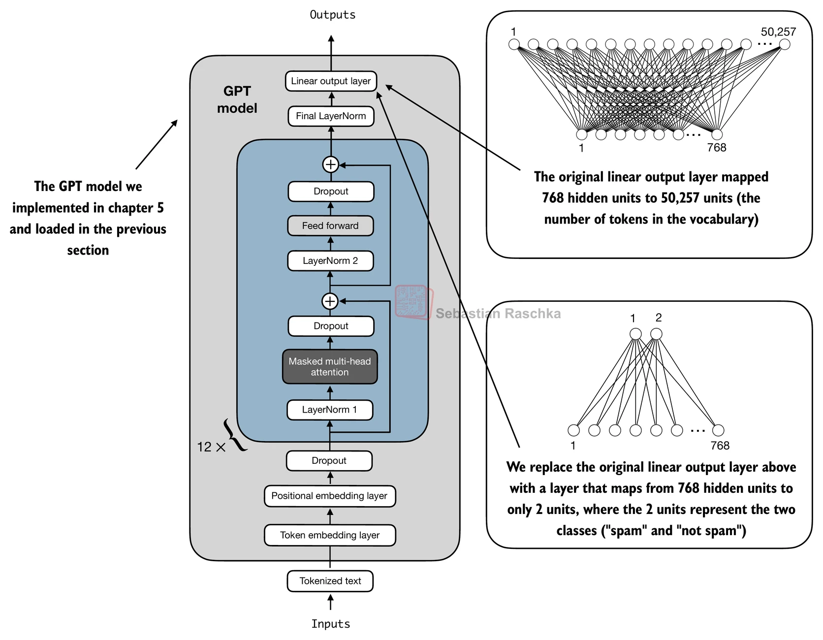
Let’s take a look at the model architecture first.
print(model)GPTModel(
(tok_emb): Embedding(50257, 768)
(pos_emb): Embedding(1024, 768)
(drop_emb): Dropout(p=0.0, inplace=False)
(trf_blocks): Sequential(
(0): TransformerBlock(
(att): MultiHeadAttention(
(W_query): Linear(in_features=768, out_features=768, bias=True)
(W_key): Linear(in_features=768, out_features=768, bias=True)
(W_value): Linear(in_features=768, out_features=768, bias=True)
(out_proj): Linear(in_features=768, out_features=768, bias=True)
(dropout): Dropout(p=0.0, inplace=False)
)
(ff): FeedForward(
(layers): Sequential(
(0): Linear(in_features=768, out_features=3072, bias=True)
(1): GELU()
(2): Linear(in_features=3072, out_features=768, bias=True)
)
)
(norm1): LayerNorm()
(norm2): LayerNorm()
(drop_resid): Dropout(p=0.0, inplace=False)
)
(1): TransformerBlock(
(att): MultiHeadAttention(
(W_query): Linear(in_features=768, out_features=768, bias=True)
(W_key): Linear(in_features=768, out_features=768, bias=True)
(W_value): Linear(in_features=768, out_features=768, bias=True)
(out_proj): Linear(in_features=768, out_features=768, bias=True)
(dropout): Dropout(p=0.0, inplace=False)
)
(ff): FeedForward(
(layers): Sequential(
(0): Linear(in_features=768, out_features=3072, bias=True)
(1): GELU()
(2): Linear(in_features=3072, out_features=768, bias=True)
)
)
(norm1): LayerNorm()
(norm2): LayerNorm()
(drop_resid): Dropout(p=0.0, inplace=False)
)
(2): TransformerBlock(
(att): MultiHeadAttention(
(W_query): Linear(in_features=768, out_features=768, bias=True)
(W_key): Linear(in_features=768, out_features=768, bias=True)
(W_value): Linear(in_features=768, out_features=768, bias=True)
(out_proj): Linear(in_features=768, out_features=768, bias=True)
(dropout): Dropout(p=0.0, inplace=False)
)
(ff): FeedForward(
(layers): Sequential(
(0): Linear(in_features=768, out_features=3072, bias=True)
(1): GELU()
(2): Linear(in_features=3072, out_features=768, bias=True)
)
)
(norm1): LayerNorm()
(norm2): LayerNorm()
(drop_resid): Dropout(p=0.0, inplace=False)
)
(3): TransformerBlock(
(att): MultiHeadAttention(
(W_query): Linear(in_features=768, out_features=768, bias=True)
(W_key): Linear(in_features=768, out_features=768, bias=True)
(W_value): Linear(in_features=768, out_features=768, bias=True)
(out_proj): Linear(in_features=768, out_features=768, bias=True)
(dropout): Dropout(p=0.0, inplace=False)
)
(ff): FeedForward(
(layers): Sequential(
(0): Linear(in_features=768, out_features=3072, bias=True)
(1): GELU()
(2): Linear(in_features=3072, out_features=768, bias=True)
)
)
(norm1): LayerNorm()
(norm2): LayerNorm()
(drop_resid): Dropout(p=0.0, inplace=False)
)
(4): TransformerBlock(
(att): MultiHeadAttention(
(W_query): Linear(in_features=768, out_features=768, bias=True)
(W_key): Linear(in_features=768, out_features=768, bias=True)
(W_value): Linear(in_features=768, out_features=768, bias=True)
(out_proj): Linear(in_features=768, out_features=768, bias=True)
(dropout): Dropout(p=0.0, inplace=False)
)
(ff): FeedForward(
(layers): Sequential(
(0): Linear(in_features=768, out_features=3072, bias=True)
(1): GELU()
(2): Linear(in_features=3072, out_features=768, bias=True)
)
)
(norm1): LayerNorm()
(norm2): LayerNorm()
(drop_resid): Dropout(p=0.0, inplace=False)
)
(5): TransformerBlock(
(att): MultiHeadAttention(
(W_query): Linear(in_features=768, out_features=768, bias=True)
(W_key): Linear(in_features=768, out_features=768, bias=True)
(W_value): Linear(in_features=768, out_features=768, bias=True)
(out_proj): Linear(in_features=768, out_features=768, bias=True)
(dropout): Dropout(p=0.0, inplace=False)
)
(ff): FeedForward(
(layers): Sequential(
(0): Linear(in_features=768, out_features=3072, bias=True)
(1): GELU()
(2): Linear(in_features=3072, out_features=768, bias=True)
)
)
(norm1): LayerNorm()
(norm2): LayerNorm()
(drop_resid): Dropout(p=0.0, inplace=False)
)
(6): TransformerBlock(
(att): MultiHeadAttention(
(W_query): Linear(in_features=768, out_features=768, bias=True)
(W_key): Linear(in_features=768, out_features=768, bias=True)
(W_value): Linear(in_features=768, out_features=768, bias=True)
(out_proj): Linear(in_features=768, out_features=768, bias=True)
(dropout): Dropout(p=0.0, inplace=False)
)
(ff): FeedForward(
(layers): Sequential(
(0): Linear(in_features=768, out_features=3072, bias=True)
(1): GELU()
(2): Linear(in_features=3072, out_features=768, bias=True)
)
)
(norm1): LayerNorm()
(norm2): LayerNorm()
(drop_resid): Dropout(p=0.0, inplace=False)
)
(7): TransformerBlock(
(att): MultiHeadAttention(
(W_query): Linear(in_features=768, out_features=768, bias=True)
(W_key): Linear(in_features=768, out_features=768, bias=True)
(W_value): Linear(in_features=768, out_features=768, bias=True)
(out_proj): Linear(in_features=768, out_features=768, bias=True)
(dropout): Dropout(p=0.0, inplace=False)
)
(ff): FeedForward(
(layers): Sequential(
(0): Linear(in_features=768, out_features=3072, bias=True)
(1): GELU()
(2): Linear(in_features=3072, out_features=768, bias=True)
)
)
(norm1): LayerNorm()
(norm2): LayerNorm()
(drop_resid): Dropout(p=0.0, inplace=False)
)
(8): TransformerBlock(
(att): MultiHeadAttention(
(W_query): Linear(in_features=768, out_features=768, bias=True)
(W_key): Linear(in_features=768, out_features=768, bias=True)
(W_value): Linear(in_features=768, out_features=768, bias=True)
(out_proj): Linear(in_features=768, out_features=768, bias=True)
(dropout): Dropout(p=0.0, inplace=False)
)
(ff): FeedForward(
(layers): Sequential(
(0): Linear(in_features=768, out_features=3072, bias=True)
(1): GELU()
(2): Linear(in_features=3072, out_features=768, bias=True)
)
)
(norm1): LayerNorm()
(norm2): LayerNorm()
(drop_resid): Dropout(p=0.0, inplace=False)
)
(9): TransformerBlock(
(att): MultiHeadAttention(
(W_query): Linear(in_features=768, out_features=768, bias=True)
(W_key): Linear(in_features=768, out_features=768, bias=True)
(W_value): Linear(in_features=768, out_features=768, bias=True)
(out_proj): Linear(in_features=768, out_features=768, bias=True)
(dropout): Dropout(p=0.0, inplace=False)
)
(ff): FeedForward(
(layers): Sequential(
(0): Linear(in_features=768, out_features=3072, bias=True)
(1): GELU()
(2): Linear(in_features=3072, out_features=768, bias=True)
)
)
(norm1): LayerNorm()
(norm2): LayerNorm()
(drop_resid): Dropout(p=0.0, inplace=False)
)
(10): TransformerBlock(
(att): MultiHeadAttention(
(W_query): Linear(in_features=768, out_features=768, bias=True)
(W_key): Linear(in_features=768, out_features=768, bias=True)
(W_value): Linear(in_features=768, out_features=768, bias=True)
(out_proj): Linear(in_features=768, out_features=768, bias=True)
(dropout): Dropout(p=0.0, inplace=False)
)
(ff): FeedForward(
(layers): Sequential(
(0): Linear(in_features=768, out_features=3072, bias=True)
(1): GELU()
(2): Linear(in_features=3072, out_features=768, bias=True)
)
)
(norm1): LayerNorm()
(norm2): LayerNorm()
(drop_resid): Dropout(p=0.0, inplace=False)
)
(11): TransformerBlock(
(att): MultiHeadAttention(
(W_query): Linear(in_features=768, out_features=768, bias=True)
(W_key): Linear(in_features=768, out_features=768, bias=True)
(W_value): Linear(in_features=768, out_features=768, bias=True)
(out_proj): Linear(in_features=768, out_features=768, bias=True)
(dropout): Dropout(p=0.0, inplace=False)
)
(ff): FeedForward(
(layers): Sequential(
(0): Linear(in_features=768, out_features=3072, bias=True)
(1): GELU()
(2): Linear(in_features=3072, out_features=768, bias=True)
)
)
(norm1): LayerNorm()
(norm2): LayerNorm()
(drop_resid): Dropout(p=0.0, inplace=False)
)
)
(final_norm): LayerNorm()
(out_head): Linear(in_features=768, out_features=50257, bias=False)
)
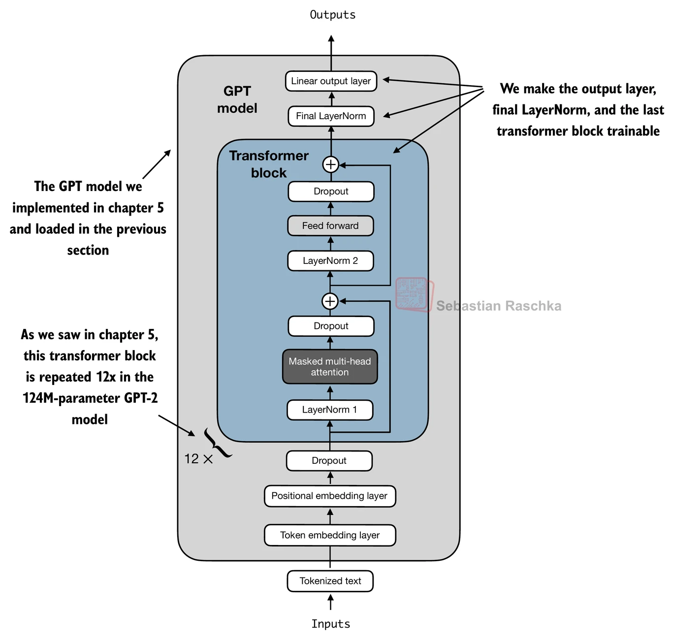
The goal is to replace and finetune ONLY the output layer. To achieve this, we first freeze the model, meaning that we make all layers non-trainable.
for param in model.parameters():
    param.requires_grad = False
Then, we replace the output layer (model.out_head), which originally maps the layer inputs to 50,257 dimensions (the size of the vocabulary).
Since we finetune the model for binary classification (predicting 2 classes, “spam” and “not spam”), we can replace the output layer as shown below, which will be trainable by default.
Note that we use
BASE_CONFIG["emb_dim"](which is equal to 768 in the"gpt2-small (124M)"model) to keep the code below more general.
torch.manual_seed(123)

num_classes = 2
model.out_head = torch.nn.Linear(in_features=BASE_CONFIG["emb_dim"], out_features=num_classes)
Technically, it’s sufficient to only train the output layer, but finetuning additional layers can noticeably improve the performance. So, we are also making the last transformer block and the final LayerNorm module connecting the last transformer block to the output layer trainable.
for param in model.trf_blocks[-1].parameters():
    param.requires_grad = True

for param in model.final_norm.parameters():
    param.requires_grad = True
For example, let’s feed it some text input:
inputs = tokenizer.encode("Do you have time")
inputs = torch.tensor(inputs).unsqueeze(0)
print("Inputs:", inputs)
print("Inputs dimensions:", inputs.shape) # shape: (batch_size, num_tokens)
Inputs: tensor([[5211, 345, 423, 640]])
Inputs dimensions: torch.Size([1, 4])
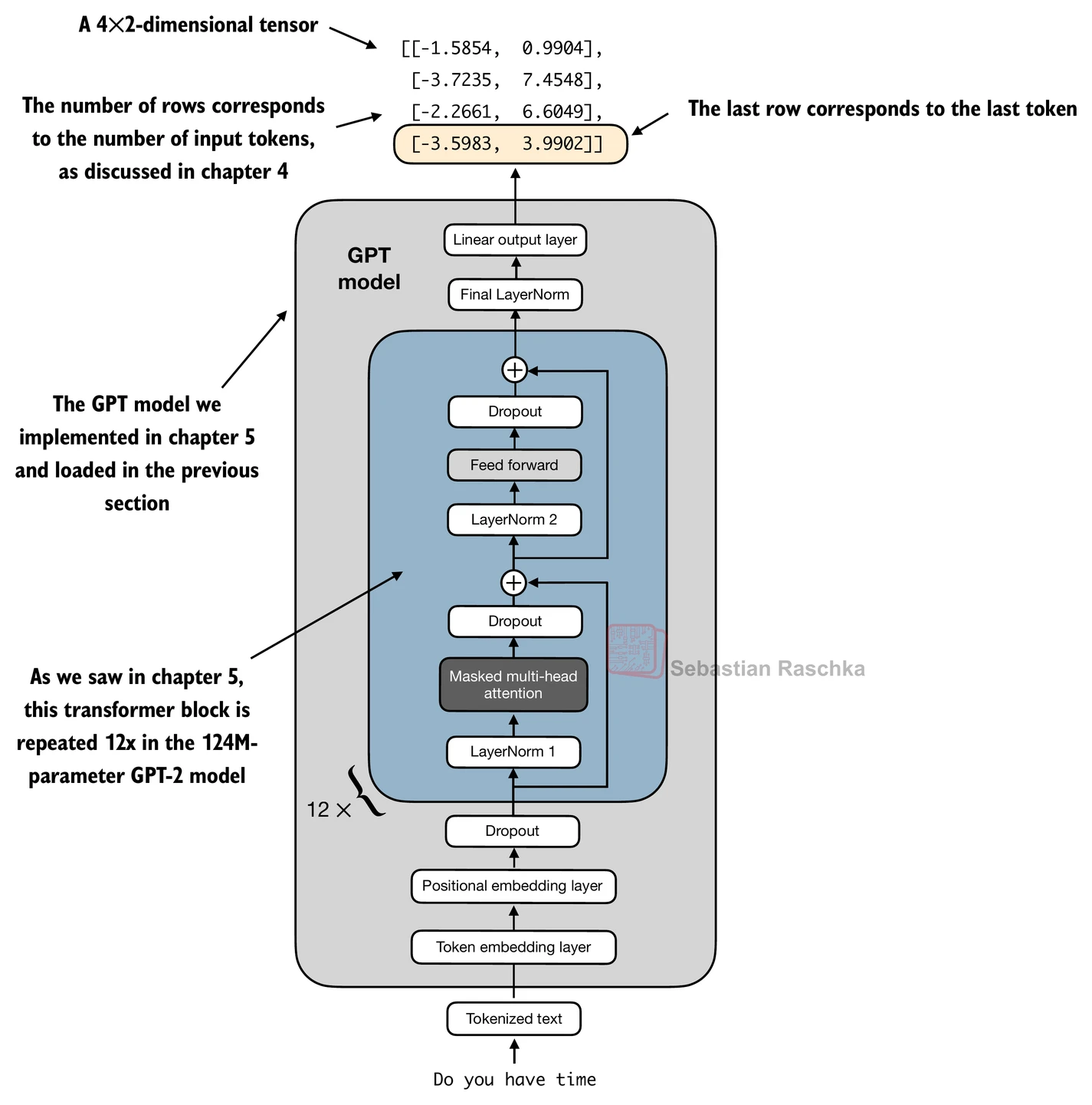
What’s different compared to previous chapters is that it now has 2 output dimensions instead of 50,257.
with torch.no_grad():
    outputs = model(inputs)

print("Outputs:\n", outputs)
print("Outputs dimensions:", outputs.shape) # shape: (batch_size, num_tokens, num_classes)
Outputs:
tensor([[[-1.5854, 0.9904],
[-3.7235, 7.4548],
[-2.2661, 6.6049],
[-3.5983, 3.9902]]])
Outputs dimensions: torch.Size([1, 4, 2])
For each input token, there’s one output vector. Since we fed the model a text sample with 4 input tokens, the output consists of 4 2-dimensional output vectors above.
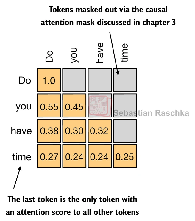
In previous chapter, we discussed the attention mechanism, which connects each input token to each other input token.
We then also introduced the causal attention mask that is used in GPT-like models; this causal mask lets a current token only attend to the current and previous token positions.
Based on this causal attention mechanism, the 4th (last) token contains the most information among all tokens because it’s the only token that includes information about all other tokens.
Hence, we are particularly interested in this last token, which we will finetune for the spam classification task.
print("Last output token:", outputs[:, -1, :])Last output token: tensor([[-3.5983, 3.9902]])
Calculating classification loss and accuracy
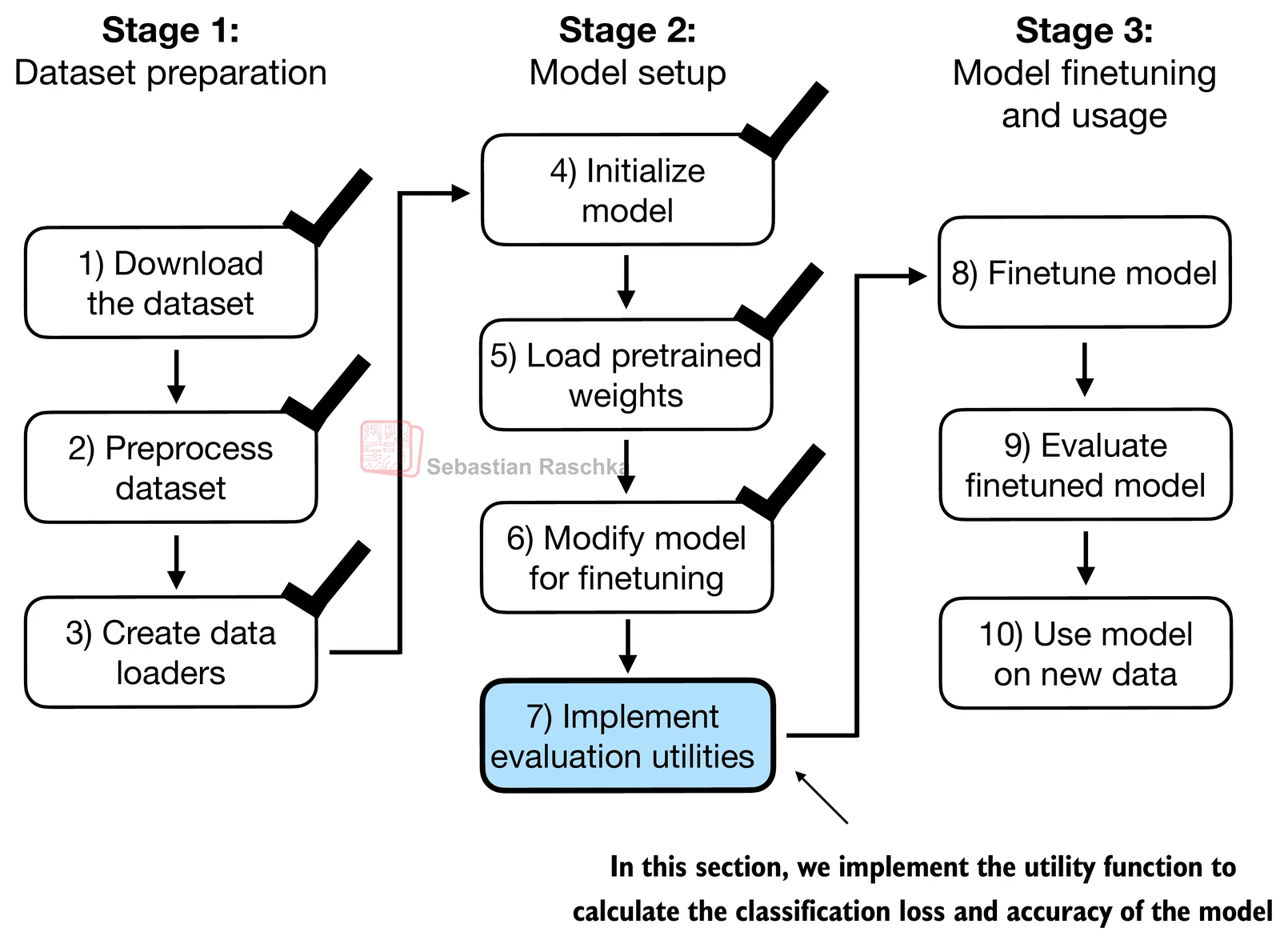
Before explaining the loss calculation, let’s have a brief look at how the model outputs are turned into class labels.
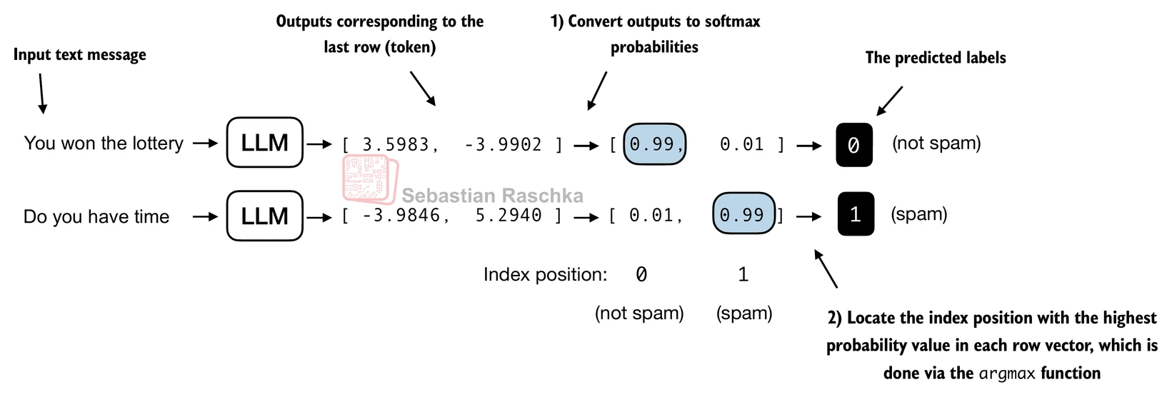
print("Last output token:", outputs[:, -1, :])Last output token: tensor([[-3.5983, 3.9902]])
We convert the outputs (logits) into probability scores via the
softmaxfunction and thenobtain the index position of the largest probability value via the
argmaxfunction.
probas = torch.softmax(outputs[:, -1, :], dim=-1)
label = torch.argmax(probas)
print("Class label:", label.item())
Class label: 1
We can apply this concept to calculate the classification accuracy.
To calculate the classification accuracy, we can apply the preceding
argmax-based prediction code to all examples in a dataset and calculate the fraction of correct predictions as follows (just like in ML):
def calc_accuracy_loader(data_loader, model, device, num_batches=None):
    model.eval()
    correct_predictions, num_examples = 0, 0

    if num_batches is None:
        num_batches = len(data_loader)
    else:
        num_batches = min(num_batches, len(data_loader))
    for i, (input_batch, target_batch) in enumerate(data_loader):
        if i < num_batches:
            input_batch, target_batch = input_batch.to(device), target_batch.to(device)

            with torch.no_grad():
                logits = model(input_batch)[:, -1, :]  # Logits of last output token
            predicted_labels = torch.argmax(logits, dim=-1)

            num_examples += predicted_labels.shape[0]
            correct_predictions += (predicted_labels == target_batch).sum().item()
        else:
            break
    return correct_predictions / num_examples
Let’s apply the function to calculate the classification accuracies for the different datasets:
if torch.cuda.is_available():
    device = torch.device("cuda")
elif torch.backends.mps.is_available():
    # Use PyTorch 2.9 or newer for stable mps results
    major, minor = map(int, torch.__version__.split(".")[:2])
    if (major, minor) >= (2, 9):
        device = torch.device("mps")
    else:
        device = torch.device("cpu")
else:
    device = torch.device("cpu")

print("Device:", device)

model.to(device) # no assignment model = model.to(device) necessary for nn.Module classes

torch.manual_seed(123) # For reproducibility due to the shuffling in the training data loader

train_accuracy = calc_accuracy_loader(train_loader, model, device, num_batches=10)
val_accuracy = calc_accuracy_loader(val_loader, model, device, num_batches=10)
test_accuracy = calc_accuracy_loader(test_loader, model, device, num_batches=10)

print(f"Training accuracy: {train_accuracy*100:.2f}%")
print(f"Validation accuracy: {val_accuracy*100:.2f}%")
print(f"Test accuracy: {test_accuracy*100:.2f}%")
Device: cuda
Training accuracy: 46.25%
Validation accuracy: 45.00%
Test accuracy: 48.75%
As we can see, the prediction accuracies are not very good, since we haven’t finetuned the model yet.
Before we can start finetuning (/training), we first have to define the loss function we want to optimize during training.
The goal is to maximize the spam classification accuracy of the model; however, classification accuracy is not a differentiable function.
Hence, instead, we minimize the cross-entropy loss as a proxy for maximizing the classification accuracy.
def calc_loss_batch(input_batch, target_batch, model, device):
    input_batch, target_batch = input_batch.to(device), target_batch.to(device)
    logits = model(input_batch)[:, -1, :]  # Logits of last output token
    loss = torch.nn.functional.cross_entropy(logits, target_batch)
    return loss
# Same as in previous chapter
def calc_loss_loader(data_loader, model, device, num_batches=None):
total_loss = 0.
if len(data_loader) == 0:
return float("nan")
elif num_batches is None:
num_batches = len(data_loader)
else:
# Reduce the number of batches to match the total number of batches in the data loader
# if num_batches exceeds the number of batches in the data loader
num_batches = min(num_batches, len(data_loader))
for i, (input_batch, target_batch) in enumerate(data_loader):
if i < num_batches:
loss = calc_loss_batch(input_batch, target_batch, model, device)
total_loss += loss.item()
else:
break
return total_loss / num_batchesUsing the calc_closs_loader, we compute the initial training, validation, and test set losses before we start training.
with torch.no_grad(): # Disable gradient tracking for efficiency because we are not training, yet
    train_loss = calc_loss_loader(train_loader, model, device, num_batches=5)
    val_loss = calc_loss_loader(val_loader, model, device, num_batches=5)
    test_loss = calc_loss_loader(test_loader, model, device, num_batches=5)

print(f"Training loss: {train_loss:.3f}")
print(f"Validation loss: {val_loss:.3f}")
print(f"Test loss: {test_loss:.3f}")
Training loss: 2.453
Validation loss: 2.583
Test loss: 2.322
Finetuning model on supervised data
In this section, we define and use the training function to improve the classification accuracy of the model.
The
train_classifier_simplefunction below is practically the same as thetrain_model_simplefunction we used for pretraining the model in previous chapter.The only differences are that we now:
Track the number of training examples seen (
examples_seen) instead of the number of tokens seen.Calculate the accuracy after each epoch instead of printing a sample text after each epoch.
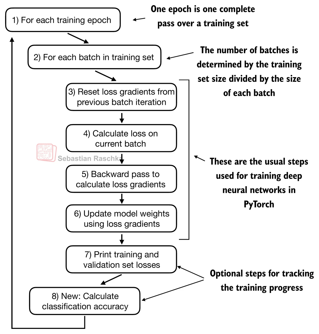
# Overall the same as `train_model_simple` in chapter 5
def train_classifier_simple(model, train_loader, val_loader, optimizer, device, num_epochs,
                            eval_freq, eval_iter):
    # Initialize lists to track losses and examples seen
    train_losses, val_losses, train_accs, val_accs = [], [], [], []
    examples_seen, global_step = 0, -1

    # Main training loop
    for epoch in range(num_epochs):
        model.train()  # Set model to training mode

        for input_batch, target_batch in train_loader:
            optimizer.zero_grad() # Reset loss gradients from previous batch iteration
            loss = calc_loss_batch(input_batch, target_batch, model, device)
            loss.backward() # Calculate loss gradients
            optimizer.step() # Update model weights using loss gradients
            examples_seen += input_batch.shape[0] # New: track examples instead of tokens
            global_step += 1

            # Optional evaluation step
            if global_step % eval_freq == 0:
                train_loss, val_loss = evaluate_model(
                    model, train_loader, val_loader, device, eval_iter)
                train_losses.append(train_loss)
                val_losses.append(val_loss)
                print(f"Ep {epoch+1} (Step {global_step:06d}): "
                      f"Train loss {train_loss:.3f}, Val loss {val_loss:.3f}")

        # Calculate accuracy after each epoch
        train_accuracy = calc_accuracy_loader(train_loader, model, device, num_batches=eval_iter)
        val_accuracy = calc_accuracy_loader(val_loader, model, device, num_batches=eval_iter)
        print(f"Training accuracy: {train_accuracy*100:.2f}% | ", end="")
        print(f"Validation accuracy: {val_accuracy*100:.2f}%")
        train_accs.append(train_accuracy)
        val_accs.append(val_accuracy)

    return train_losses, val_losses, train_accs, val_accs, examples_seen
The evaluate_model function used in the train_classifier_simple is the same as the one we used in previous chapter.
# Same as previous chapter
def evaluate_model(model, train_loader, val_loader, device, eval_iter):
    model.eval()
    with torch.no_grad():
        train_loss = calc_loss_loader(train_loader, model, device, num_batches=eval_iter)
        val_loss = calc_loss_loader(val_loader, model, device, num_batches=eval_iter)
    model.train()
    return train_loss, val_loss
The training takes a while, depends on your device.
import time

start_time = time.time()

torch.manual_seed(123)

optimizer = torch.optim.AdamW(model.parameters(), lr=5e-5, weight_decay=0.1)

num_epochs = 5
train_losses, val_losses, train_accs, val_accs, examples_seen = train_classifier_simple(
    model, train_loader, val_loader, optimizer, device,
    num_epochs=num_epochs, eval_freq=50, eval_iter=5,
)

end_time = time.time()
execution_time_minutes = (end_time - start_time) / 60
print(f"Training completed in {execution_time_minutes:.2f} minutes.")
Ep 1 (Step 000000): Train loss 2.153, Val loss 2.392
Ep 1 (Step 000050): Train loss 0.617, Val loss 0.637
Ep 1 (Step 000100): Train loss 0.523, Val loss 0.557
Training accuracy: 70.00% | Validation accuracy: 72.50%
Ep 2 (Step 000150): Train loss 0.561, Val loss 0.489
Ep 2 (Step 000200): Train loss 0.419, Val loss 0.397
Ep 2 (Step 000250): Train loss 0.409, Val loss 0.353
Training accuracy: 82.50% | Validation accuracy: 85.00%
Ep 3 (Step 000300): Train loss 0.333, Val loss 0.320
Ep 3 (Step 000350): Train loss 0.340, Val loss 0.306
Training accuracy: 90.00% | Validation accuracy: 90.00%
Ep 4 (Step 000400): Train loss 0.136, Val loss 0.200
Ep 4 (Step 000450): Train loss 0.153, Val loss 0.132
Ep 4 (Step 000500): Train loss 0.222, Val loss 0.137
Training accuracy: 100.00% | Validation accuracy: 97.50%
Ep 5 (Step 000550): Train loss 0.207, Val loss 0.143
Ep 5 (Step 000600): Train loss 0.083, Val loss 0.074
Training accuracy: 100.00% | Validation accuracy: 97.50%
Training completed in 1.05 minutes.
We use matplotlib to plot the loss function for the training and validation set.
import matplotlib.pyplot as plt

def plot_values(epochs_seen, examples_seen, train_values, val_values, label="loss"):
    fig, ax1 = plt.subplots(figsize=(5, 3))

    # Plot training and validation loss against epochs
    ax1.plot(epochs_seen, train_values, label=f"Training {label}")
    ax1.plot(epochs_seen, val_values, linestyle="-.", label=f"Validation {label}")
    ax1.set_xlabel("Epochs")
    ax1.set_ylabel(label.capitalize())
    ax1.legend()

    # Create a second x-axis for examples seen
    ax2 = ax1.twiny()  # Create a second x-axis that shares the same y-axis
    ax2.plot(examples_seen, train_values, alpha=0)  # Invisible plot for aligning ticks
    ax2.set_xlabel("Examples seen")

    fig.tight_layout()  # Adjust layout to make room
    plt.savefig(f"{label}-plot.pdf")
    plt.show()
epochs_tensor = torch.linspace(0, num_epochs, len(train_losses))
examples_seen_tensor = torch.linspace(0, examples_seen, len(train_losses))
plot_values(epochs_tensor, examples_seen_tensor, train_losses, val_losses)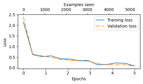
Above, based on the downward slope, we see that the model learns well.
Similarly, we can plot the accuracy below.
epochs_tensor = torch.linspace(0, num_epochs, len(train_accs))
examples_seen_tensor = torch.linspace(0, examples_seen, len(train_accs))

plot_values(epochs_tensor, examples_seen_tensor, train_accs, val_accs, label="accuracy")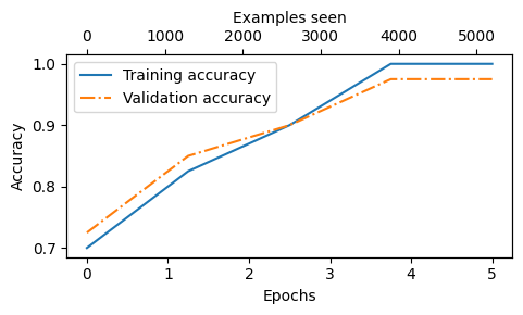
However, we have to keep in mind that we specified eval_iter=5 in the training function earlier, which means that we only estimated the training and validation set performances.
train_accuracy = calc_accuracy_loader(train_loader, model, device)
val_accuracy = calc_accuracy_loader(val_loader, model, device)
test_accuracy = calc_accuracy_loader(test_loader, model, device)

print(f"Training accuracy: {train_accuracy*100:.2f}%")
print(f"Validation accuracy: {val_accuracy*100:.2f}%")
print(f"Test accuracy: {test_accuracy*100:.2f}%")
Training accuracy: 97.21%
Validation accuracy: 97.32%
Test accuracy: 95.67%
However, based on the slightly lower test set performance, we can see that the model overfits the training data to a very small degree, as well as the validation data that has been used for tweaking some of the hyperparameters, such as the learning rate.
This is normal, however, and this gap could potentially be further reduced by increasing the model’s dropout rate (drop_rate) or the weight_decay in the optimizer setting.
Using LLM as spam classifier
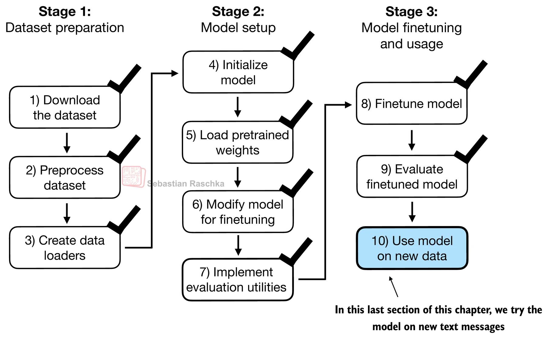
Finally, let’s use the finetuned GPT model in action.
The
classify_reviewfunction below implements the data preprocessing steps similar to theSpamDatasetwe implemented earlier.Then, the function returns the predicted integer class label from the model and returns the corresponding class name.
def classify_review(text, model, tokenizer, device, max_length=None, pad_token_id=50256):
    model.eval()

    # Prepare inputs to the model
    input_ids = tokenizer.encode(text)
    supported_context_length = model.pos_emb.weight.shape[0]
    # Note: In the book, this was originally written as pos_emb.weight.shape[1] by mistake
    # It didn't break the code but would have caused unnecessary truncation (to 768 instead of 1024)

    # Truncate sequences if they too long
    input_ids = input_ids[:min(max_length, supported_context_length)]
    assert max_length is not None, (
        "max_length must be specified. If you want to use the full model context, "
        "pass max_length=model.pos_emb.weight.shape[0]."
    )
    assert max_length <= supported_context_length, (
        f"max_length ({max_length}) exceeds model's supported context length ({supported_context_length})."
    )
    # Alternatively, a more robust version is the following one, which handles the max_length=None case better
    # max_len = min(max_length,supported_context_length) if max_length else supported_context_length
    # input_ids = input_ids[:max_len]

    # Pad sequences to the longest sequence
    input_ids += [pad_token_id] * (max_length - len(input_ids))
    input_tensor = torch.tensor(input_ids, device=device).unsqueeze(0) # add batch dimension

    # Model inference
    with torch.no_grad():
        logits = model(input_tensor)[:, -1, :]  # Logits of the last output token
    predicted_label = torch.argmax(logits, dim=-1).item()

    # Return the classified result
    return "spam" if predicted_label == 1 else "not spam"
Let’s try it out on a few examples below.
text_1 = (
    "You are a winner you have been specially"
    " selected to receive $1000 cash or a $2000 award."
)

print(classify_review(
    text_1, model, tokenizer, device, max_length=train_dataset.max_length
))
spam
text_2 = (
    "Hey, just wanted to check if we're still on"
    " for dinner tonight? Let me know!"
)

print(classify_review(
    text_2, model, tokenizer, device, max_length=train_dataset.max_length
))
not spam
Finally, let’s save the model in case we want to reuse the model later without having to train it again.
torch.save(model.state_dict(), "review_classifier.pth")Then, in a new session, we could load the model as follows:
model_state_dict = torch.load("review_classifier.pth", map_location=device, weights_only=True)
model.load_state_dict(model_state_dict)
<All keys matched successfully>