Chapter 13: Going Deeper -- the Mechanics of PyTorch (Part 2/2)¶

Prework¶

Import essentials¶

from IPython.display import Image
%matplotlib inline

Check package version (optional)¶

Add folder to path in order to load from the check_packages.py script.

import sys
sys.path.insert(0, '..')

Check recommended package versions.

from python_environment_check import check_packages


d = {
    'numpy': '1.21.2',
    'pandas': '1.3.2',
    'sklearn': '1.0',
    'torch': '1.8',
    'torchvision': '0.9.0'
}
check_packages(d)

[OK] Your Python version is 3.8.0 (tags/v3.8.0:fa919fd, Oct 14 2019, 19:37:50) [MSC v.1916 64 bit (AMD64)]
[OK] numpy 1.22.3
[OK] pandas 2.0.3
[OK] sklearn 1.3.2
[OK] torch 2.1.1+cpu
[OK] torchvision 0.16.1+cpu

Table of Contents¶

import numpy as np
import torch
import torch.nn as nn
import pandas as pd

from IPython.display import Image

13.6.Project one - predicting the fuel efficiency of a car¶

In this section, we will work on a real-world project of predicting the fuel efficiency of a car in miles per gallon (MPG). We will cover the underlying steps in machine learning tasks, such as data preprocessing, feature engineering, training, prediction (inference), and evaluation.

13.6.1.Working with feature columns¶

In machine learning and deep learning applications, we can encounter various different types of features:

continuous
unordered categorical (nominal)
ordered categorical (ordinal)

Note that while numeric data can be either continuous or discrete, in the context of machine learning with PyTorch, “numeric” data specifically refers to continuous data of floating point type.

Sometimes, feature sets are comprised of a mixture of different feature types. For example, consider a scenario with a set of seven different features, as shown in the following figure.

The features shown in the figure (model year, cylinders, displacement, horsepower, weight, acceleration, and origin) were obtained from the Auto MPG dataset, which is a common machine learning benchmark dataset for predicting the fuel efficiency of a car in MPG.

Image(filename='figures/13_07.png', width=700)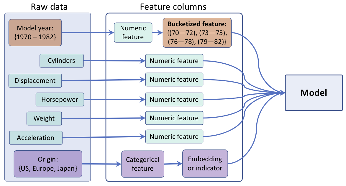

We are going to treat five features from the Auto MPG dataset (number of cylinders, displacement, horsepower, weight, and acceleration) as “numeric” (here, continuous) features. The model year can be regarded as an ordered categorical (ordinal) feature. Lastly, the manufacturing origin can be regarded as an unordered categorical (nominal) feature with three possible discrete values, 1, 2, and 3, which correspond to the US, Europe, and Japan, respectively.

Let’s first load the data.

url = 'http://archive.ics.uci.edu/ml/machine-learning-databases/auto-mpg/auto-mpg.data'
column_names = ['MPG', 'Cylinders', 'Displacement', 'Horsepower', 'Weight',
                'Acceleration', 'Model Year', 'Origin']

df = pd.read_csv(url, names=column_names,
                 na_values = "?", comment='\t',
                 sep=" ", skipinitialspace=True)

df.tail()

Then we check how many Na are in the rows (incomplete rows), and we drop them.

print(df.isna().sum())

df = df.dropna()
df = df.reset_index(drop=True)
df.tail()

MPG             0
Cylinders       0
Displacement    0
Horsepower      6
Weight          0
Acceleration    0
Model Year      0
Origin          0
dtype: int64

We need to partition the dataset into training and test datasets via sklearn.model_selection.

import sklearn
import sklearn.model_selection


df_train, df_test = sklearn.model_selection.train_test_split(df, train_size=0.8, random_state=1)
train_stats = df_train.describe().transpose()
train_stats

And we also need to standardize the continuous features.

The pandas DataFrame that we created via the previous code snippet contains five columns with values of the type float. These columns will constitute the continuous features.

numeric_column_names = ['Cylinders', 'Displacement', 'Horsepower', 'Weight', 'Acceleration']

df_train_norm, df_test_norm = df_train.copy(), df_test.copy()

for col_name in numeric_column_names:
    mean = train_stats.loc[col_name, 'mean']
    std  = train_stats.loc[col_name, 'std']
    df_train_norm.loc[:, col_name] = (df_train_norm.loc[:, col_name] - mean)/std
    df_test_norm.loc[:, col_name] = (df_test_norm.loc[:, col_name] - mean)/std
    
df_train_norm.tail()

Next, let’s group the rather fine-grained model year (ModelYear) information into buckets to simplify the learning task for the model that we are going to train later. Concretely, we are going to assign each car into one of four year buckets, as follows:

\text { bucket }= \begin{cases}0 & \text { if year }<73 \\ 1 & \text { if 73 } \leq \text { year }<76 \\ 2 & \text { if 76 } \leq \text { year }<79 \\ 3 & \text { if year } \geq 79\end{cases}

(1)

Note that the chosen intervals were selected arbitrarily to illustrate the concepts of “bucketing.” In order to group the cars into these buckets, we will first define three cut-off values: $[73,76,79]$ for the model year feature. These cut-off values are used to specify half-closed intervals, for instance, $(-\infty, 73)$ , $[73,76),[76,79)$ , and $[76, \infty)$ . Then, the original numeric features will be passed to the torch.bucketize function to generate the indices of the buckets.

We add this bucketized feature column to the Python list numeric_column_names.

boundaries = torch.tensor([73, 76, 79])
 
v = torch.tensor(df_train_norm['Model Year'].values)
df_train_norm['Model Year Bucketed'] = torch.bucketize(v, boundaries, right=True)

v = torch.tensor(df_test_norm['Model Year'].values)
df_test_norm['Model Year Bucketed'] = torch.bucketize(v, boundaries, right=True)

numeric_column_names.append('Model Year Bucketed')

Next, we will proceed with defining a list for the unordered categorical feature, Origin. In PyTorch, There are two ways to work with a categorical feature:

Using an embedding layer via nn.Embedding
- The embedding layer maps each index to a vector of random numbers of the type float, which can be trained. (You can think of the embedding layer as a more efficient implementation of a one-hot encoding multiplied with a trainable weight matrix.)
- When the number of categories is large, using the embedding layer with fewer dimensions than the number of categories can improve the performance.
Using one-hot-encoded vectors (also called indicator) via one_hot
- For example, index 0 will be encoded as $[1,0,0]$ , index 1 will be encoded as $[0,1,0]$ , and so on.

In the following code snippet, we will use the one-hot-encoding approach on the categorical feature in order to convert it into the dense format.

from torch.nn.functional import one_hot


total_origin = len(set(df_train_norm['Origin']))

origin_encoded = one_hot(torch.from_numpy(df_train_norm['Origin'].values) % total_origin)
x_train_numeric = torch.tensor(df_train_norm[numeric_column_names].values)
x_train = torch.cat([x_train_numeric, origin_encoded], 1).float()
 
origin_encoded = one_hot(torch.from_numpy(df_test_norm['Origin'].values) % total_origin)
x_test_numeric = torch.tensor(df_test_norm[numeric_column_names].values)
x_test = torch.cat([x_test_numeric, origin_encoded], 1).float()

After encoding the categorical feature into a three-dimensional dense feature, we concatenated it with the numeric features we processed in the previous step. Finally, we will create the label tensors from the ground truth MPG values as follows.

y_train = torch.tensor(df_train_norm['MPG'].values).float()
y_test = torch.tensor(df_test_norm['MPG'].values).float()

13.6.2.Training a DNN regression model¶

Now, after constructing the mandatory features and labels, we will create a data loader that uses a batch size of 8 for the train data.

from torch.utils.data import DataLoader, TensorDataset


train_ds = TensorDataset(x_train, y_train)
batch_size = 8
torch.manual_seed(1)
train_dl = DataLoader(train_ds, batch_size, shuffle=True)

Next, we will build a model with two fully connected layers where one has 8 hidden units and another has 4.

hidden_units = [8, 4]
input_size = x_train.shape[1]

all_layers = []
for hidden_unit in hidden_units:
    layer = nn.Linear(input_size, hidden_unit)
    all_layers.append(layer)
    all_layers.append(nn.ReLU())
    input_size = hidden_unit

all_layers.append(nn.Linear(hidden_units[-1], 1))

model = nn.Sequential(*all_layers)

model

Sequential(
  (0): Linear(in_features=9, out_features=8, bias=True)
  (1): ReLU()
  (2): Linear(in_features=8, out_features=4, bias=True)
  (3): ReLU()
  (4): Linear(in_features=4, out_features=1, bias=True)
)

After defining the model, we will define the MSE loss function for regression and use stochastic gradient descent for optimization.

loss_fn = nn.MSELoss()
optimizer = torch.optim.SGD(model.parameters(), lr=0.001)

Now we will train the model for 200 epochs and display the train loss for every 20 epochs.

torch.manual_seed(1)
num_epochs = 200
log_epochs = 20 
for epoch in range(num_epochs):
    loss_hist_train = 0
    for x_batch, y_batch in train_dl:
        pred = model(x_batch)[:, 0]
        loss = loss_fn(pred, y_batch)
        loss.backward()
        optimizer.step()
        optimizer.zero_grad()
        loss_hist_train += loss.item()
    if epoch % log_epochs==0:
        print(f'Epoch {epoch}  Loss {loss_hist_train/len(train_dl):.4f}')

Epoch 0  Loss 536.1047
Epoch 20  Loss 8.4361
Epoch 40  Loss 7.8695
Epoch 60  Loss 7.1891
Epoch 80  Loss 6.7064
Epoch 100  Loss 6.7603
Epoch 120  Loss 6.3107
Epoch 140  Loss 6.6884
Epoch 160  Loss 6.7549
Epoch 180  Loss 6.2029

After 200 epochs, the train loss was around 5. We can now evaluate the regression performance of the trained model on the test dataset. To predict the target values on new data points, we can feed their features to the model.

Result explanation

The MSE on the test set is 9.6, and the mean absolute error (MAE) is 2.1.

with torch.no_grad():
    pred = model(x_test.float())[:, 0]
    loss = loss_fn(pred, y_test)
    print(f'Test MSE: {loss.item():.4f}')
    print(f'Test MAE: {nn.L1Loss()(pred, y_test).item():.4f}')

Test MSE: 9.5907
Test MAE: 2.1177

13.7.Project two - classifying MNIST hand-written digits¶

We are going to load the MNIST dataset using the torchvision module.

The setup step includes loading the dataset and specifying hyperparameters (the size of the train set and test set, and the size of mini-batches). Here, we constructed a data loader with batches of 64 samples.

import torchvision 
from torchvision import transforms 


image_path = './'
transform = transforms.Compose([transforms.ToTensor()])

mnist_train_dataset = torchvision.datasets.MNIST(root=image_path, 
                                           train=True, 
                                           transform=transform, 
                                           download=True)
mnist_test_dataset = torchvision.datasets.MNIST(root=image_path, 
                                           train=False, 
                                           transform=transform, 
                                           download=False)
 
batch_size = 64
torch.manual_seed(1)
train_dl = DataLoader(mnist_train_dataset, batch_size, shuffle=True)

Downloading http://yann.lecun.com/exdb/mnist/train-images-idx3-ubyte.gz

2.6%

Downloading http://yann.lecun.com/exdb/mnist/train-images-idx3-ubyte.gz to ./MNIST\raw\train-images-idx3-ubyte.gz

100.0%

Extracting ./MNIST\raw\train-images-idx3-ubyte.gz to ./MNIST\raw

Downloading http://yann.lecun.com/exdb/mnist/train-labels-idx1-ubyte.gz

100.0%

Downloading http://yann.lecun.com/exdb/mnist/train-labels-idx1-ubyte.gz to ./MNIST\raw\train-labels-idx1-ubyte.gz
Extracting ./MNIST\raw\train-labels-idx1-ubyte.gz to ./MNIST\raw

Downloading http://yann.lecun.com/exdb/mnist/t10k-images-idx3-ubyte.gz


19.9%

Downloading http://yann.lecun.com/exdb/mnist/t10k-images-idx3-ubyte.gz to ./MNIST\raw\t10k-images-idx3-ubyte.gz

100.0%

Extracting ./MNIST\raw\t10k-images-idx3-ubyte.gz to ./MNIST\raw

Downloading http://yann.lecun.com/exdb/mnist/t10k-labels-idx1-ubyte.gz

100.0%

Downloading http://yann.lecun.com/exdb/mnist/t10k-labels-idx1-ubyte.gz to ./MNIST\raw\t10k-labels-idx1-ubyte.gz
Extracting ./MNIST\raw\t10k-labels-idx1-ubyte.gz to ./MNIST\raw

We preprocess the input features and the labels. The features in this project are the pixels of the images we read from Step 1. We defined a custom transformation using torchvision.transforms.Compose (in preceding code snippets). In this simple case, our transformation consisted only of one method, ToTensor(). The ToTensor() method converts the pixel features into a floating type tensor and also normalizes the pixels from the $[0,255]$ to $[0,1]$ range. The labels are integers from 0 to 9 representing ten digits. Hence, we don’t need to do any scaling or further conversion. Note that we can access the raw pixels using the data attribute, and don’t forget to scale them to the range $[0,1]$ .
Construct the NN model.
- Note that the model starts with a flatten layer (nn.Flatten()) that flattens an input image into a one-dimensional tensor. This is because the input images are in the shape of [1, 28, 28]. The model has two hidden layers, with 32 and 16 units respectively. And it ends with an output layer of ten units representing ten classes, activated by a softmax function.

hidden_units = [32, 16]
image_size = mnist_train_dataset[0][0].shape
input_size = image_size[0] * image_size[1] * image_size[2]

all_layers = [nn.Flatten()]
for hidden_unit in hidden_units:
    layer = nn.Linear(input_size, hidden_unit)
    all_layers.append(layer)
    all_layers.append(nn.ReLU())
    input_size = hidden_unit

all_layers.append(nn.Linear(hidden_units[-1], 10))
model = nn.Sequential(*all_layers)

model

Sequential(
  (0): Flatten(start_dim=1, end_dim=-1)
  (1): Linear(in_features=784, out_features=32, bias=True)
  (2): ReLU()
  (3): Linear(in_features=32, out_features=16, bias=True)
  (4): ReLU()
  (5): Linear(in_features=16, out_features=10, bias=True)
)

We used the cross-entropy loss function for multiclass classification and the Adam optimizer for gradient descent. We trained the model for 20 epochs and displayed the train accuracy for every epoch.

loss_fn = nn.CrossEntropyLoss()
optimizer = torch.optim.Adam(model.parameters(), lr=0.001)

torch.manual_seed(1)
num_epochs = 20
for epoch in range(num_epochs):
    accuracy_hist_train = 0
    for x_batch, y_batch in train_dl:
        pred = model(x_batch)
        loss = loss_fn(pred, y_batch)
        loss.backward()
        optimizer.step()
        optimizer.zero_grad()
        is_correct = (torch.argmax(pred, dim=1) == y_batch).float()
        accuracy_hist_train += is_correct.sum()
    accuracy_hist_train /= len(train_dl.dataset)
    print(f'Epoch {epoch}  Accuracy {accuracy_hist_train:.4f}')

Epoch 0  Accuracy 0.8531
Epoch 1  Accuracy 0.9287
Epoch 2  Accuracy 0.9413
Epoch 3  Accuracy 0.9506
Epoch 4  Accuracy 0.9558
Epoch 5  Accuracy 0.9592
Epoch 6  Accuracy 0.9627
Epoch 7  Accuracy 0.9650
Epoch 8  Accuracy 0.9674
Epoch 9  Accuracy 0.9690
Epoch 10  Accuracy 0.9710
Epoch 11  Accuracy 0.9729
Epoch 12  Accuracy 0.9739
Epoch 13  Accuracy 0.9750
Epoch 14  Accuracy 0.9764
Epoch 15  Accuracy 0.9777
Epoch 16  Accuracy 0.9779
Epoch 17  Accuracy 0.9798
Epoch 18  Accuracy 0.9806
Epoch 19  Accuracy 0.9813

We will evaluate the training set on the testing set.

pred = model(mnist_test_dataset.data / 255.)
is_correct = (torch.argmax(pred, dim=1) == mnist_test_dataset.targets).float()
print(f'Test accuracy: {is_correct.mean():.4f}')

Test accuracy: 0.9647

Readers may ignore the next cell.

! python ../.convert_notebook_to_script.py --input ch13_part2.ipynb --output ch13_part2.py

[NbConvertApp] Converting notebook ch13_part2.ipynb to script
[NbConvertApp] Writing 7052 bytes to ch13_part2.py