Chapter 12 - Parallelizing Neural Network Training with PyTorch (Part 1/2)¶

Prework¶

Import essentials¶

Check package version (optional)¶

Add folder to path in order to load from the check_packages.py script.

Check recommended package versions.

Watermark (optional)¶

Optional watermark extension is a small IPython notebook plugin that I developed to make the code reproducible.

You can install watermark Jupyter extension via

conda install watermark -c conda-forge  

or

pip install watermark   

For more information, please see: https://github.com/rasbt/watermark.

Table of Contents¶

• 12.1.PyTorch and training performance

  • 12.1.1.Performance challenges

  • 12.1.2.What is PyTorch?

  • 12.1.3.How we will learn PyTorch

• 12.2.First steps with PyTorch

  • 12.2.1.Installing PyTorch

  • 12.2.2.Creating tensors in PyTorch

  • 12.2.3.Manipulating the data type and shape of a tensor

  • 12.2.4.Applying mathematical operations to tensors

  • 12.2.5.Split, stack, and concatenate tensors

• 12.3.Building input pipelines in PyTorch

  • 12.3.1.Creating a PyTorch DataLoader from existing tensors

  • 12.3.2.Combining two tensors into a joint dataset

  • 12.3.3.Shuffle, batch, and repeat

  • 12.3.4.Creating a dataset from files on your local storage disk

  • 12.3.5.Fetching available datasets from the torchvision.datasets library

12.1.PyTorch and training performance¶

12.1.1.Performance challenges¶

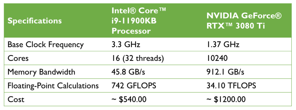
12.1.2.What is PyTorch?¶

• PyTorch is built around a computation graph composed of a set of nodes.

• Each node represents an operation that may have zero or more inputs or outputs.

• Tensors in PyTorch are similar to NumPy’s arrays, except that tensors are optimized for automatic differentiation and can run on GPUs.

• Tensors can be understood as a generalization of scalars, vectors, matrices, and so on.

  • scalar: rank-0 tensor

  • vector: rank-1 tensor

  • matrix: rank-2 tensor

  • matrices stack in 3rd dimension: rank-3 tensors

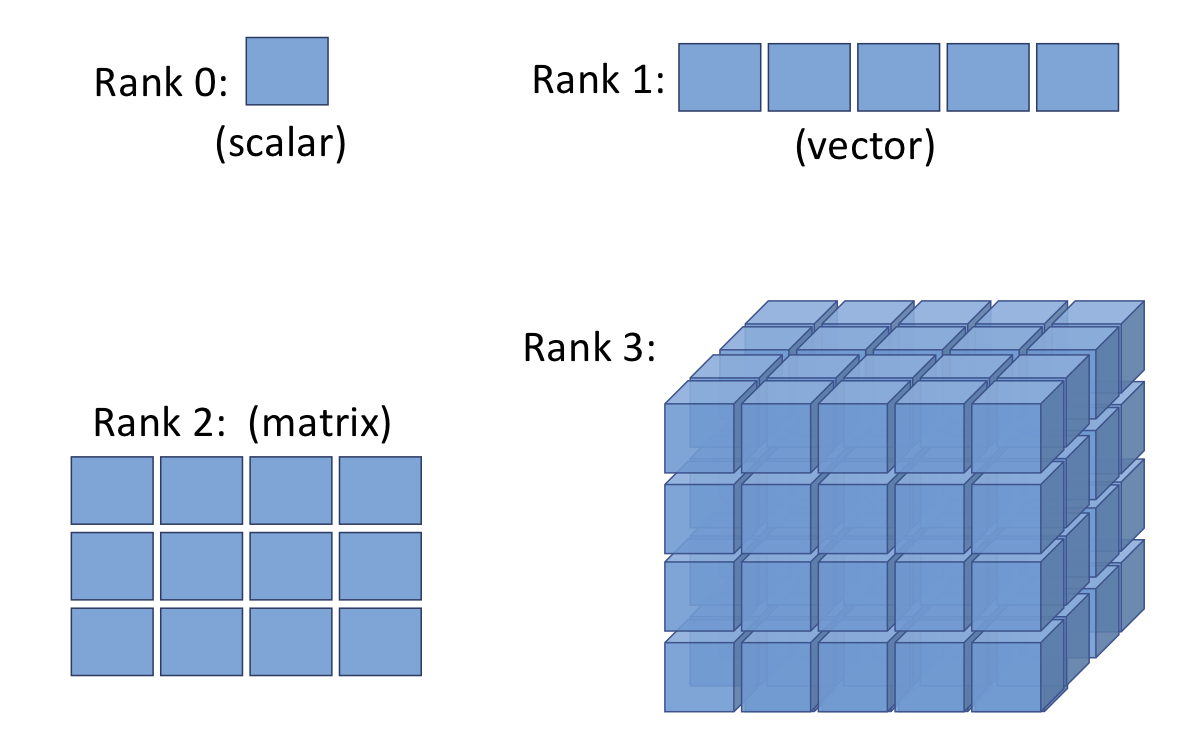
12.1.3.How we will learn PyTorch¶

No code provided.

12.2.First steps with PyTorch¶

12.2.1.Installing PyTorch¶

12.2.2.Creating tensors in PyTorch¶

Firstly, we can simply create a tensor from a list or a NumPy array using the torch.tensor or the torch.from_numpy function as follows.

Similar to NumPy arrays, we can also see these properties.

Finally, creating a tensor of random values can be done as follows.

12.2.3.Manipulating the data type and shape of a tensor¶

The torch.to() function can be used to change the data type of a tensor to a desired type.

Certain operations require that the input tensors have a certain number of dimensions (that is, rank) associated with a certain number of elements (shape). Thus, we might need to change the shape of a tensor, add a new dimension, or squeeze an unnecessary dimension. PyTorch provides useful functions (or operations) to achieve this:

1. Transposing a tensor.

2. Reshaping a tensor (for example, from a 1D vector to a 2D array).

3. Removing the unnecessary dimensions (dimensions that have size 1, which are not needed).

12.2.4.Applying mathematical operations to tensors¶

In this subsection, we will cover some widely used linear algebra operations. First, let’s instantiate two random tensors, one with uniform distribution in the range [–1, 1) and the other with a standard normal distribution.

Note that torch.rand returns a tensor filled with random numbers from a uniform distribution in the range of [0, 1). Also, notice that t1 and t2 have the same shape.

Now, to compute the element-wise product of t1 and t2, we can use the following.

The mean of each column in t1 can be computed as follows.

The matrix-matrix product between t1 and t2 (that is, $t_1 \times t_2^{\mathrm{T}}$, where the superscript T is for transpose) can be computed by using the torch.matmul() function as follows.

On the other hand, computing $t_1^T \times t_2$ is performed by transposing t1, resulting in an array of size 2×2.

Finally, the torch.linalg.norm() function is useful for computing the $L^p$ norm of a tensor. For example, we can calculate the $L^2$ norm of t1 as follows.

To verify that this code snippet computes the $L^2$ norm of t1 correctly, you can compare the results with the following NumPy function.

12.2.5.Split, stack, and concatenate tensors¶

Assume that we have a single tensor, and we want to split it into two or more tensors. For this, PyTorch provides a convenient torch.chunk() function, which divides an input tensor into a list of equally sized tensors. We can determine the desired number of splits as an integer using the chunks argument to split a tensor along the desired dimension specified by the dim argument. In this case, the total size of the input tensor along the specified dimension must be divisible by the desired number of splits. Alternatively, we can provide the desired sizes in a list using the torch.split() function. Let’s have a look at an example of both these options:

1. Providing the number of splits: torch.chunk()

   • In this example, a tensor of size 6 was divided into a list of three tensors each with size 2. If the tensor size is not divisible by the chunks value, the last chunk will be smaller.

2. Providing the sizes of different splits: torch.split()

   • Alternatively, instead of defining the number of splits, we can also specify the sizes of the output tensors directly. Here, we are splitting a tensor of size 5 into tensors of sizes 3 and 2.

Sometimes, we are working with multiple tensors and need to concatenate or stack them to create a single tensor. In this case, PyTorch functions such as torch.stack() and torch.cat() come in handy.

1. Concatenate tensors: torch.cat()

   • For example, let’s create a 1D tensor, A, containing 1s with size 3, and a 1D tensor, B, containing 0s with size 2, and concatenate them into a 1D tensor, C, of size 5.

2. Stack tensors: torch.stack()

   • If we create 1D tensors A and B, both with size 3, then we can stack them together to form a 2D tensor, S.

12.3.Building input pipelines in PyTorch¶

12.3.1.Creating a PyTorch DataLoader from existing tensors¶

If the data already exists in the form of a tensor object, a Python list, or a NumPy array, we can easily create a dataset loader using the torch.utils.data.DataLoader() class. It returns an object of the DataLoader class, which we can use to iterate through the individual elements in the input dataset. As a simple example, consider the following code, which creates a dataset from a list of values from 0 to 5.

We can easily iterate through a dataset entry by entry as follows.

If we want to create batches from this dataset, with a desired batch size of 3, we can do this with the batch_size argument as follows. The optional drop_last argument is useful for cases when the number of elements in the tensor is not divisible by the desired batch size. The default value for drop_last is False.

12.3.2.Combining two tensors into a joint dataset¶

Often, we may have the data in two (or possibly more) tensors. For example, we could have a tensor for features and a tensor for labels. In such cases, we need to build a dataset that combines these tensors, which will allow us to retrieve the elements of these tensors in tuples.

Note that a common source of error could be that the element-wise correspondence between the original features ($x$) and labels ($y$) might be lost (for example, if the two datasets are shuffled separately). However, once they are merged into one dataset, it is safe to apply these operations.

Assume that we have two tensors, t_x and t_y:

• t_x holds our feature values, each of size 3

• t_y stores the class labels

We want to create a joint dataset from these two tensors. We first need to create a Dataset class as follows. A custom Dataset class must contain the following methods to be used by the data loader later on:

• __init__(): This is where the initial logic happens, such as reading existing arrays, loading a file, filtering data, and so forth.

• __getitem__(): This returns the corresponding sample to the given index.

Then we create a joint dataset of t_x and t_y with the custom Dataset class and print each example of the joint dataset as follows.

We can also simply utilize the torch.utils.data.TensorDataset class, if the second dataset is a labeled dataset in the form of tensors. So, instead of using our self-defined Dataset class, JointDataset, we can create a joint dataset as follows.

12.3.3.Shuffle, batch, and repeat¶

When training an NN model using stochastic gradient descent optimization, it is important to feed training data as randomly shuffled batches. You have already seen how to specify the batch size using the batch_size argument of a data loader object. Now, in addition to creating batches, you will see how to shuffle and reiterate over the datasets. We will continue working with the previous joint dataset.

First, let’s create a shuffled version data loader from the joint_dataset dataset. Here, each batch contains two data records ($x$) and the corresponding labels ($y$). Now we iterate through the data loader entry by entry.

Result explanation

The rows are shuffled without losing the one-to-one correspondence between the entries in x and y.

In addition, when training a model for multiple epochs, we need to shuffle and iterate over the dataset by the desired number of epochs. So, let’s iterate over the batched dataset twice.

Result explanation

• The first epoch:

  • the first batch contains a pair of values [y=1, y=2], and the second batch contains a pair of values [y=3, y=0].

• The second epoch:

  • two batches contain a pair of values, [y=2, y=0] and [y=1, y=3] respectively. For each iteration, the elements within a batch are also shuffled.

12.3.4.Creating a dataset from files on your local storage disk¶

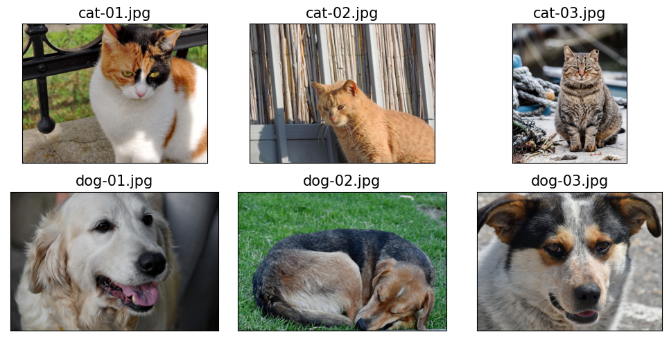
In this section, we will build a dataset from image files stored on disk. There is an image folder associated with the online content of this chapter. After downloading the folder, you should be able to see six images of cats and dogs in JPEG format.

This small dataset will show how building a dataset from stored files generally works. To accomplish this, we are going to use two additional modules:

1. Image in PIL to read the image file contents

2. transforms in torchvision to decode the raw contents and resize the images

Before we start, let’s take a look at the content of these files. We will use the pathlib library to generate a list of image files.

Next, we will visualize these image examples using Matplotlib.

Result explanation

Just from this visualization and the printed image shapes, we can already see that the images have different aspect ratios. If you print the aspect ratios (or data array shapes) of these images, you will see that some images are 900 pixels high and 1200 pixels wide $(900 \times 1200)$, some are $800 \times 1200$, and one is $900 \times 742$. Later, we will preprocess these images to a consistent size.

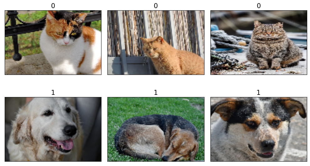
Another point to consider is that the labels for these images are provided within their filenames. So, we extract these labels from the list of filenames, assigning label 1 to dogs and label 0 to cats.

Now, we have two lists:

1. a list of filenames (or paths of each image)

2. a list of their labels

In the previous section, you learned how to create a customized joint dataset from two arrays, we are going to create a joint dataset for them, where the joint dataset has filenames and labels.

Next, we need to apply transformations to this dataset:

• load the image content from its file path

• decode the raw content

• resize it to a desired size, for example, $80 \times 120$

As mentioned before, we use the torchvision.transforms module to resize the images and convert the loaded pixels into tensors as follows.

Now we update the ImageDataset class with the transform we just defined.

The __getitem__ method in the ImageDataset class wraps all four steps into a single function, including:

• the loading of the raw content (images and labels)

• decoding the images into tensors

• resizing the images.

The function then returns a dataset that we can iterate over and apply other operations that we learned about in the previous sections via a data loader, such as shuffling and batching.

Finally, we visualize these transformed image examples using Matplotlib. This results in the following visualization of the retrieved example images, along with their labels.

12.3.5.Fetching available datasets from the torchvision.datasets library¶

Fetching CelebA dataset

1. Downloading the image files manually

   • You can try setting download=True below. If this results in a BadZipfile error, we recommend downloading the img_align_celeba.zip file manually from http://mmlab.ie.cuhk.edu.hk/projects/CelebA.html. In the Google Drive folder, you can find it under the Img folder as shown below:

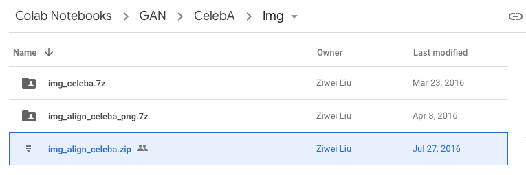
• You can also try this direct link: https://drive.google.com/file/d/0B7EVK8r0v71pZjFTYXZWM3FlRnM/view?usp=sharing&resourcekey=0-dYn9z10tMJOBAkviAcfdyQ

• After downloading, please put this file into the ./celeba subolder and unzip it.

2. Next, you need to download the annotation files and put them into the same ./celeba subfolder. The annotation files can be found under Anno:

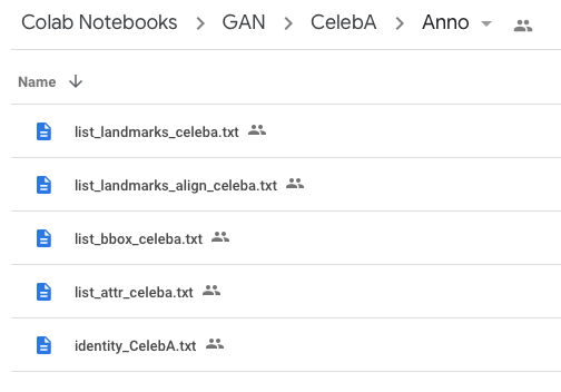
• direct links are provided below:

  • identity_CelebA.txt

  • list_attr_celeba.txt

  • list_bbox_celeba.txt

  • list_landmarks_align_celeba.txt

  • list_landmarks_celeba.txt

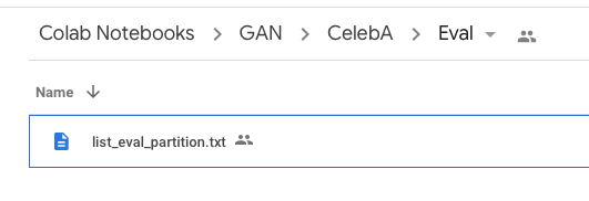
3. Lastly, you need to download the file list_eval_partition.txt and place it under ./celeba:

• list_eval_partition.txt

After completing steps 1-3 above, please ensure you have the following files in your ./celeba subfolder, and the files are non-empty (that is, they have similar file sizes as shown below):

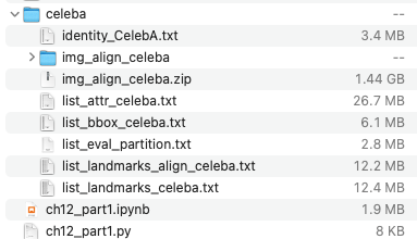
The following paragraphs include two different datasets: 1. CelebA dataset 2. MINST dataset

1. CelebA dataset

The torchvision.datasets library provides a nice collection of freely available image datasets for training or evaluating deep learning models. Similarly, the torchtext.datasets library provides datasets for natural language. Here, we use torchvision.datasets as an example.

Let’s first work with the CelebA dataset with torchvision.datasets.CelebA. The description of torchvision.datasets.CelebA provides some useful information to help us understand the structure of this dataset:

• The database has three subsets, 'train', 'valid', and 'test'.

  • We can select a specific subset or load all of them with the split parameter.

• The images are stored in PIL.Image format.

  • We can obtain a transformed version using a custom transform function, such as transforms.ToTensor and transforms.Resize.

• There are different types of targets we can use, including 'attributes', 'identity', and 'landmarks'.

  • 'attributes' is 40 facial attributes for the person in the image, such as facial expression, makeup, hair properties ...

  • 'identity' is the person ID for an image.

  • 'landmarks' refers to the dictionary of extracted facial points, such as the position of the eyes, nose ...

Next, we will call the torchvision.datasets.CelebA class to download the data, store it on disk in a designated folder, and load it into a torch.utils.data.Dataset object. After we have instantiated the datasets, let’s check if the object is of the torch.utils.data.Dataset class via function isinstance().

As mentioned, the dataset is already split into train, test, and validation datasets, and we only load the train set. And we only use the 'attributes' target. In order to see what the data examples look like, we can execute the following code.

Note that the sample in this dataset comes in a tuple of (PIL.Image, attributes). If we want to pass this dataset to a supervised deep learning model during training, we have to reformat it as a tuple of (features tensor, label). For the label, we will use the 'Smiling' category from the attributes as an example, which is the 31st element.

Finally, let’s take the first 18 examples from it to visualize them with their 'Smiling' labels, which are retrieved from celeba_dataset.

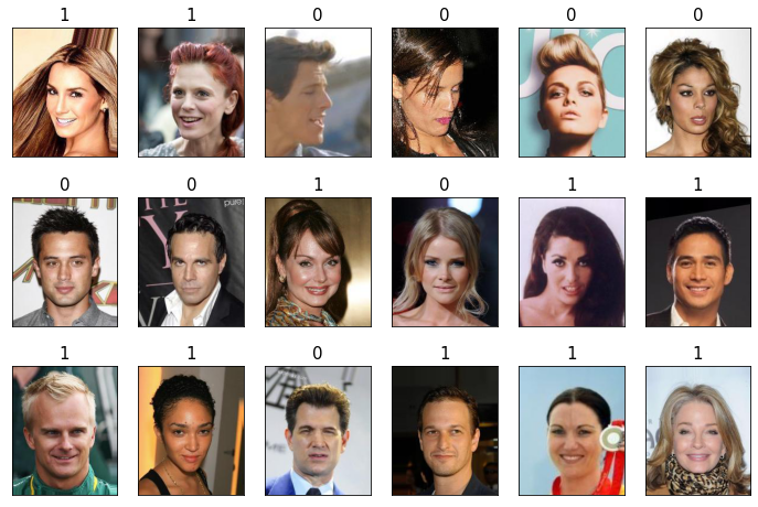
2. MINST dataset

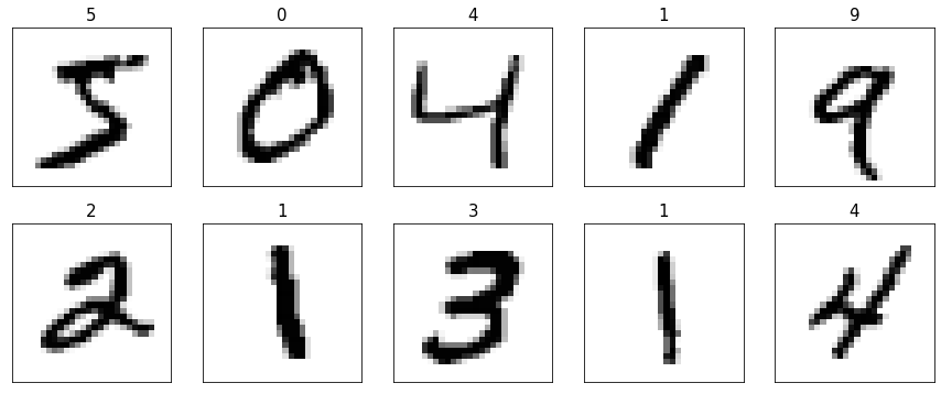
Next, we will proceed with the second dataset from torchvision.datasets.MNIST. Let’s see how it can be used to fetch the MNIST digit dataset:

• The database has two partitions, 'train' and 'test'.

  • We need to select a specific subset to load.

• The images are stored in PIL.Image format.

  • We can obtain a transformed version using a custom transform function, such as transforms.ToTensor and transforms.Resize.

• There are 10 classes for the target, from 0 to 9.

Now, we can download the ‘train’ partition, convert the elements to tuples, and visualize 10 examples.

Readers may ignore the next cell.