Chapter 13: Going Deeper -- the Mechanics of PyTorch (Part 1/2)¶

Prework¶

Import essentials¶

Check package version (optional)¶

Add folder to path in order to load from the check_packages.py script.

Check recommended package versions.

Watermark (optional)¶

Optional watermark extension is a small IPython notebook plugin that I developed to make the code reproducible.

You can install watermark Jupyter extension via

conda install watermark -c conda-forge  

or

pip install watermark   

For more information, please see: https://github.com/rasbt/watermark.

Table of Contents¶

• 13.1.The key features of PyTorch

• 13.2.PyTorch’s computation graphs

  • 13.2.1.Understanding computation graphs

  • 13.2.2.Creating a graph in PyTorch

• 13.3.PyTorch tensor objects for storing and updating model parameters

• 13.4.Computing gradients via automatic differentiation

  • 13.4.1.Computing the gradients of the loss with respect to trainable variables

  • 13.4.2.Understanding automatic differentiation

  • 13.4.3.Adversarial examples

• 13.5.Simplifying implementations of common architectures via the torch.nn module

  • 13.5.1.Implementing models based on nn.Sequential

  • 13.5.2.Choosing a loss function

  • 13.5.3.Solving an XOR classification problem

  • 13.5.4.Making model building more flexible with nn.Module

  • 13.5.5.Writing custom layers in PyTorch

13.1.The key features of PyTorch¶

No code provided.

13.2.PyTorch’s computation graphs¶

13.2.1.Understanding computation graphs¶

PyTorch relies on building a computation graph at its core, and it uses this computation graph to derive relationships between tensors from the input all the way to the output. PyTorch builds this computation graph and uses it to compute the gradients accordingly.

Let’s say that we have rank 0 (scalar) tensors $a, b$, and $c$ and we want to evaluate $z=2 \times(a-b)+c$.

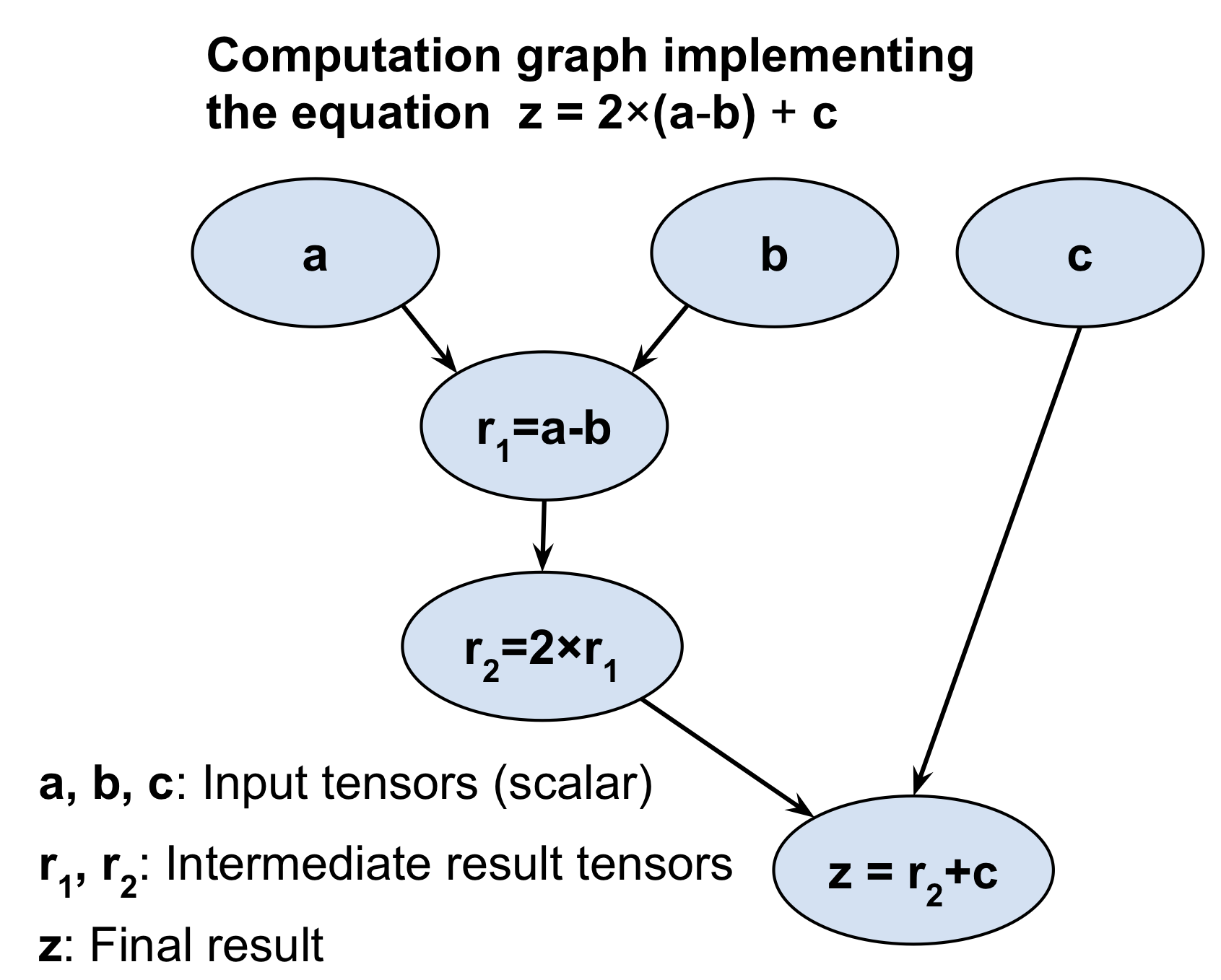
13.2.2.Creating a graph in PyTorch¶

Let’s look at a simple example that illustrates how to create a graph in PyTorch for evaluating $z=2 \times(a-b)+c$, as shown in the previous figure. The variables $a, b$, and $c$ are scalars (single numbers), and we define these as PyTorch tensors. To create the graph, we can simply define a regular Python function with a, b, and c as its input arguments.

Now, to carry out the computation, we can simply call this function with tensor objects as function arguments. Note that PyTorch functions such as add, sub (or subtract), and mul (or multiply) also allow us to provide inputs of higher ranks in the form of a PyTorch tensor object. In the following code example, we provide scalar inputs (rank-0), as well as rank-1 and rank 2 inputs.

13.3.PyTorch Tensor objects for storing and updating model parameters¶

In PyTorch, a special tensor object for which gradients need to be computed allows us to store and update the parameters of our models during training. Such a tensor can be created by just assigning requires_grad to True on user-specified initial values.

Notice that requires_grad is set to False by default. This value can be efficiently set to True by running requires_grad_().

Xavier initialization

You will recall that for NN models, initializing model parameters with random weights is necessary to break the symmetry during backpropagation - otherwise, a multilayer NN would be no more useful than a single-layer NN like logistic regression. When creating a PyTorch tensor, we can also use a random initialization scheme. PyTorch can generate random numbers based on a variety of probability distributions (see https://pytorch.org/docs/stable/torch.html#random-sampling). In the following example, we will take a look at some standard initialization methods that are also available in the torch.nn.init module (see https://pytorch.org/docs/stable/nn.init.html).

So, let’s look at how we can create a tensor with Xavier initialization, which is a classic random initialization scheme that was proposed by Xavier Glorot and Yoshua Bengio. For this, we first create an empty tensor and an operator called init as an object of class GlorotNormal. Then, we fill this tensor with values according to the Xavier initialization by calling the xavier_normal_() method. In the following example, we initialize a tensor of shape $2 \times 3$.

13.4.Computing gradients via automatic differentiation¶

As you already know, optimizing NNs requires computing the gradients of the loss with respect to the NN weights. This is required for optimization algorithms such as stochastic gradient descent (SGD). In addition, gradients have other applications, such as diagnosing the network to find out why an NN model is making a particular prediction for a test example. Therefore, in this section, we will cover how to compute gradients of a computation with respect to its input variables.

13.4.1.Computing the gradients of the loss with respect to trainable variables¶

PyTorch supports automatic differentiation, which can be thought of as an implementation of the chain rule for computing gradients of nested functions. Note that for the sake of simplicity, we will use the term gradient to refer to both partial derivatives and gradients.

Let’s work with a simple example where we will compute $z=w x+b$ and define as follows:

• feature = $x$

• target = $y$

• prediction = $z$

• the squared loss = $(y-z)^2$

In the more general case, where we may have multiple predictions and targets, we compute the loss as the sum of the squared error, $Loss=\sum_i\left(y_i-z_i\right)^2$ .

In order to implement this computation in PyTorch, we will define the model parameters, $w$ and $b$, as variables (tensors with the requires_gradient = True), and the input, $x$ and $y$, as default tensors. We will compute the loss tensor and use it to compute the gradients of the model parameters, $w$ and $b$.

Computing the value $z$ is a forward pass in an NN. We used the backward method on the loss tensor to compute $\frac{\partial \text { Loss }}{\partial w}$ and $\frac{\partial \text { Loss }}{\partial b}$.

Since this is a very simple example, we can obtain $\frac{\partial \text { Loss }}{\partial w}=2 x(w x+b-y)$ symbolically to verify that the computed gradients match the results we obtained in the previous code example.

13.4.2.Understanding automatic differentiation¶

Automatic differentiation represents a set of computational techniques for computing gradients of arbitrary arithmetic operations. During this process, gradients of a computation (expressed as a series of operations) are obtained by accumulating the gradients through repeated applications of the chain rule. To better understand the concept behind automatic differentiation, let’s consider a series of nested computations, $y=f(g(h(x)))$, with input $x$ and output $y$. This can be broken into a series of steps:

• $u_0=x$

• $u_1=h(x)$

• $u_2=g\left(u_1\right)$

• $u_3=f\left(u_2\right)=y$

The derivative $\frac{d y}{d x}$ can be computed in two different ways:

1. forward accumulation, which starts with $\frac{d u_3}{d x}=\frac{d u_3}{d u_2} \frac{d u_2}{d u_0}$

2. reverse accumulation, which starts with $\frac{d y}{d u_0}=\frac{d y}{d u_1} \frac{d u_1}{d u_0}$

Note that PyTorch uses the latter, reverse accumulation, which is more efficient for implementing backpropagation.

13.4.3.Adversarial examples¶

Computing gradients of the loss with respect to the input example is used for generating adversarial examples (or adversarial attacks). In computer vision, adversarial examples are examples that are generated by adding some small, imperceptible noise (or perturbations) to the input example, which results in a deep NN misclassifying them.

13.5.Simplifying implementations of common architectures via the torch.nn module¶

13.5.1.Implementing models based on nn.Sequential¶

With nn.Sequential, the layers stored inside the model are connected in a cascaded way. In the following example, we will build a model with two densely (fully) connected layers.

We specified the layers and instantiated the model after passing the layers to the nn.Sequential class. The output of the first fully connected layer is used as the input to the first ReLU layer. The output of the first ReLU layer becomes the input for the second fully connected layer. Finally, the output of the second fully connected layer is used as the input to the second ReLU layer.

Configure layers

We can further configure these layers, for example, by applying different activation functions, initializers, or regularization methods to the parameters. A comprehensive and complete list of available options for most of these categories can be found in the official documentation:

• Choosing activation functions: https://pytorch.org/docs/stable/nn.html#non-linearactivations-weighted-sum-nonlinearity

• Initializing the layer parameters via nn.init: https://pytorch.org/docs/stable/nn.init. html

• Applying L2 regularization to the layer parameters (to prevent overfitting) via the parameter weight_decay of some optimizers in torch.optim: https://pytorch.org/docs/stable/optim.html

• Applying L1 regularization to the layer parameters (to prevent overfitting) by adding the L1 penalty term to the loss tensor.

In the following code example, we will configure the first fully connected layer by specifying the initial value distribution for the weight with Xavier initialization. Then, we will configure the second fully connected layer by computing the L1 penalty term for the weight matrix.

13.5.2.Choosing a loss function¶

Regarding the choices for optimization algorithms, SGD and Adam are the most widely used methods. The choice of loss function depends on the task. For example, you might use mean square error loss for a regression problem; the family of cross-entropy loss functions supplies the possible choices for classification task.

Furthermore, you can use the appropriate metrics for the problem. For example, precision and recall, accuracy, area under the curve (AUC), and false negative and false positive scores are appropriate metrics for evaluating classification models.

In this example, we will use the SGD optimizer, and cross-entropy loss for binary classification.

13.5.3.Solving an XOR classification problem¶

Next, we will look at a more practical example: solving the classic XOR classification problem. First, we will use the nn.Sequential() class to build the model. Along the way, you will also learn about the capacity of a model for handling nonlinear decision boundaries. Then, we will cover building a model via nn.Module that will give us more flexibility and control over the layers of the network.

The XOR classification problem is a classic problem for analyzing the capacity of a model with regard to capturing the nonlinear decision boundary between two classes. We generate a toy dataset of 200 training examples with two features $\left(x_0, x_1\right)$ drawn from a uniform distribution between $[-1,1)$. Then, we assign the ground truth label for training example $i$ according to the following rule:

The code for generating the data and splitting it into the training and validation datasets is as follows.

• 50% for training dataset (100 training examples)

• 25% for testing dataset

• 25% for validation dataset

Result explanation

The code results in the following scatterplot of the training and validation examples, shown with different markers based on their class label.

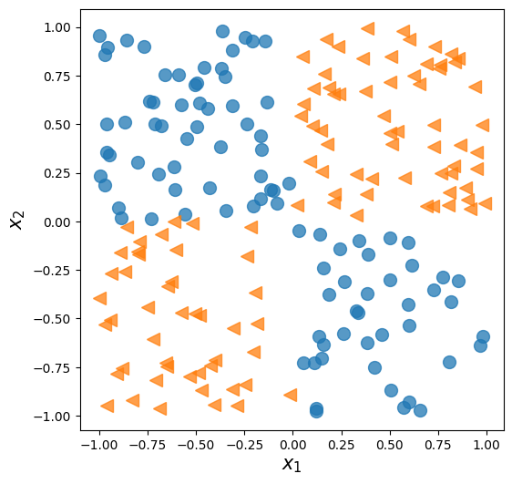
We now need to decide what architecture we should choose for this task and dataset. As a general rule of thumb, the more layers we have, and the more neurons we have in each layer, the larger the capacity of the model will be. Here, the model capacity can be thought of as a measure of how readily the model can approximate complex functions. While having more parameters means the network can fit more complex functions, larger models are usually harder to train (and prone to overfitting). In practice, it is always a good idea to start with a simple model as a baseline, for example, a single-layer NN like logistic regression.

After defining the model, we will initialize the cross-entropy loss function for binary classification and the SGD optimizer.

Next, we will create a data loader that uses a batch size of 2 for the train data.

Now we will train the model for 200 epochs and record a history of training epochs.

Result explanation

This results in the following figure, with two separate panels for the losses and accuracies.

As you can see, a simple model with no hidden layer can only derive a linear decision boundary, which is unable to solve the XOR problem. As a consequence, we can observe that the loss terms for both the training and the validation datasets are very high, and the classification accuracy is very low.

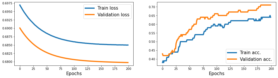
Nonlinear decision boundary for better classification

To derive a nonlinear decision boundary, we can add one or more hidden layers connected via nonlinear activation functions. The universal approximation theorem states that a feedforward NN with a single hidden layer and a relatively large number of hidden units can approximate arbitrary continuous functions relatively well. Thus, one approach for tackling the XOR problem more satisfactorily is to add a hidden layer and compare different numbers of hidden units until we observe satisfactory results on the validation dataset. Adding more hidden units would correspond to increasing the width of a layer.

Alternatively, we can also add more hidden layers, which will make the model deeper. The advantage of making a network deeper rather than wider is that fewer parameters are required to achieve a comparable model capacity.

However, a downside of deep (versus wide) models is that deep models are prone to vanishing and exploding gradients, which make them harder to train.

As an exercise, try adding one, two, three, and four hidden layers, each with four hidden units. In the following example, we will take a look at the results of a feedforward NN with two hidden layers.

Result explanation

Now, we can see that the model is able to derive a nonlinear decision boundary for this data, and the model reaches 100 percent accuracy on the training dataset. The validation dataset’s accuracy is 95 percent, which indicates that the model is slightly overfitting.

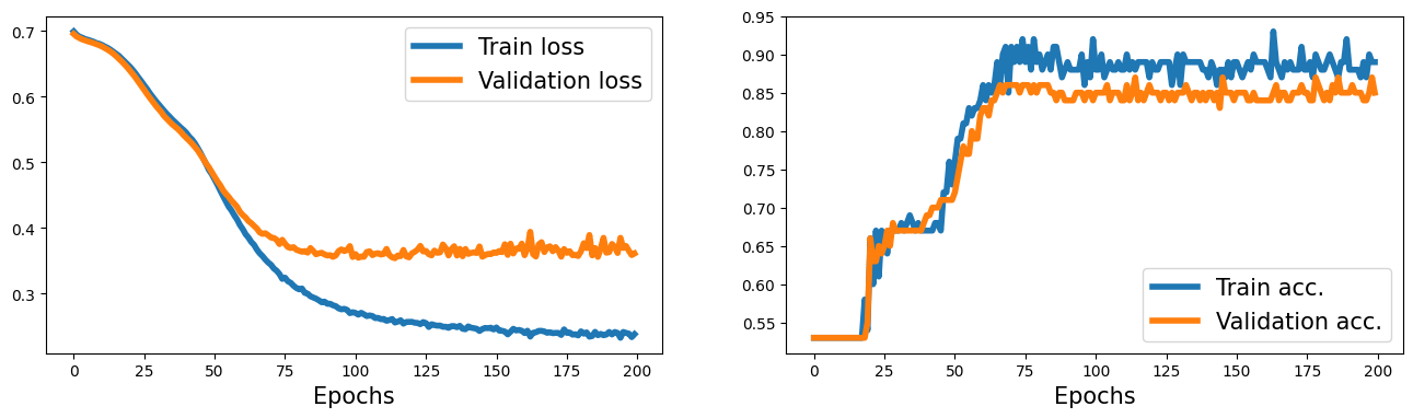
13.5.4.Making model building more flexible with nn.Module¶

In the previous example, we used the PyTorch Sequential class to create a fully connected NN with multiple layers. This is a very common and convenient way of building models. However, it unfortunately doesn’t allow us to create more complex models that have multiple input, output, or intermediate branches. That’s where nn.Module comes in handy.

The alternative way to build complex models is by subclassing nn.Module. In this approach, we create a new class derived from nn.Module and define the method,

• __init__()

  • We define the layers as attributes of the class so that they can be accessed via the self reference attribute.

• forward()

  • We specify how these layers are to be used in the forward pass of the NN.

• predict()

  • To compute the decision boundary of our model.

  • It will return the predicted class (0 or 1) for a sample.

Notice that we put all layers in the nn.ModuleList object, which is just a list object composed of nn.Module items.

Once we define an instance of this new class, we can train it as we did previously.

Next, besides the train history, we will use the mlxtend library to visualize the validation data and the decision boundary. The following code will plot the training performance along with the decision region bias.

Result explanation

This results with three separate panels for the losses, accuracies, and the scatterplot of the validation examples, along with the decision boundary.

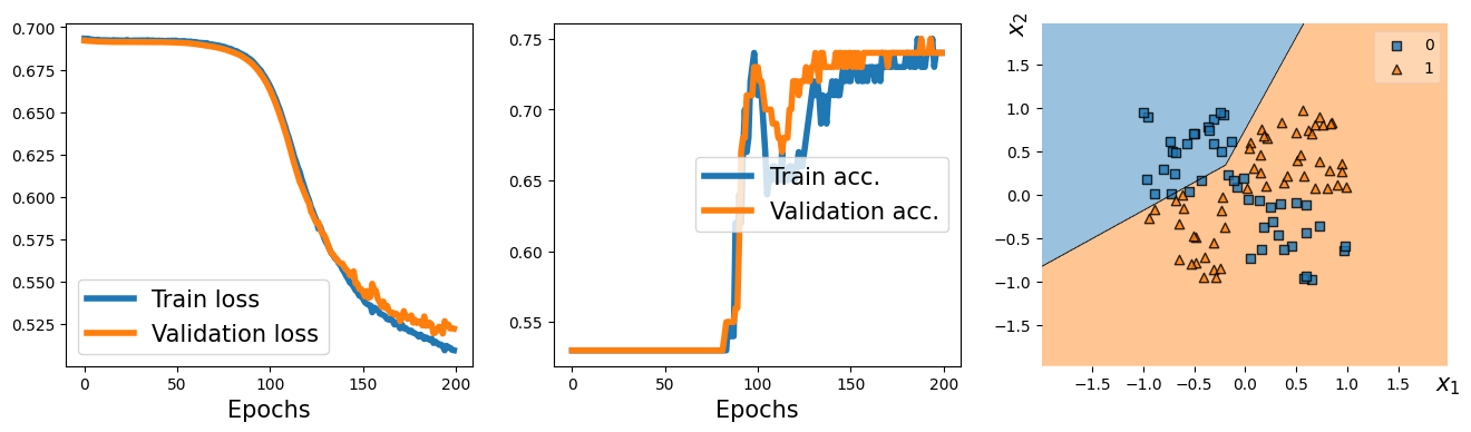
13.5.5.Writing custom layers in PyTorch¶

In cases where we want to define a new layer that is not already supported by PyTorch, we can define a new class derived from the nn.Module class. This is especially useful when designing a new layer or customizing an existing layer.

To illustrate the concept of implementing custom layers, let’s consider a simple example. Imagine we want to define a new linear layer that computes $w(x+\epsilon)+b$, where $\epsilon$ refers to a random variable as a noise variable. To implement this computation, we define a new class as a subclass of nn.Module. For this new class, NoiseyLinear, we define:

• __init__()

  • In the constructor, we define the variables and other required tensors for our customized layer. We can create variables and initialize them in the constructor if the input_size is given to the constructor. Alternatively, we can delay the variable initialization (for instance, if we do not know the exact input shape upfront) and delegate it to another method for late variable creation.

  • noise_stddev, to specify the standard deviation for the distribution of $\epsilon$, which is sampled from a Gaussian distribution.

• forward()

  • training=False, to distinguish whether the layer is used during training or only for prediction (this is sometimes also called inference) or evaluation.

Note that the random vector, $\epsilon$, was to be generated and added to the input during training only and not used for inference or evaluation.

Before we go a step further and use our custom NoisyLinear layer in a model, let’s test it in the context of a simple example.

1. In the following code, we will define a new instance of this layer, and execute it on an input tensor. Then, we will call the layer three times on the same input tensor:

2. Now, let’s create a new model similar to the previous one for solving the XOR classification task, MyNoisyModule. As before, we will use the nn.Module class for model building, but this time, we will use our NoisyLinear layer as the first hidden layer of the multilayer perceptron. The code is as follows:

3. Similarly, we will train the model as we did previously. At this time, to compute the prediction on the training batch, we use pred = model(x_batch, True)[:, 0] instead of pred = model(x_batch)[:, 0]:

4. After the model is trained, we can plot the losses, accuracies, and the decision boundary:

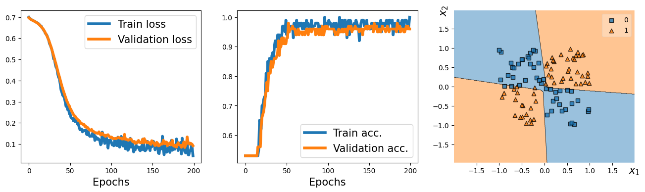
Readers may ignore the next cell.