Chapter 12 - Parallelizing Neural Network Training with PyTorch (Part 2/2)¶

Prework¶

Import essentials¶

from IPython.display import Image
%matplotlib inline

Check package version (optional)¶

Add folder to path in order to load from the check_packages.py script.

import sys
sys.path.insert(0, '..')

Check recommended package versions.

from python_environment_check import check_packages


d = {
    'numpy': '1.21.2',
    'matplotlib': '3.4.3',
    'torch': '1.9.0',
}
check_packages(d)

[OK] numpy 1.22.3
[OK] matplotlib 3.5.1
[OK] torch 2.1.1+cpu

Watermark (optional)¶

Optional watermark extension is a small IPython notebook plugin that I developed to make the code reproducible.

You can install watermark Jupyter extension via

conda install watermark -c conda-forge

pip install watermark

For more information, please see: https://github.com/rasbt/watermark.

%load_ext watermark
%watermark -a "Sebastian Raschka, Johnny Yu" -u -d -v -p numpy,pandas,matplotlib,scipy,sklearn

The watermark extension is already loaded. To reload it, use:
  %reload_ext watermark
Author: Sebastian Raschka, Johnny Yu

Last updated: 2023-12-16

Python implementation: CPython
Python version       : 3.8.0
IPython version      : 8.12.2

numpy     : 1.22.3
pandas    : 2.0.3
matplotlib: 3.5.1
scipy     : 1.8.0
sklearn   : 1.3.2

Table of Contents¶

12.4.Building a neural network model in PyTorch¶

12.4.1.The PyTorch neural network module (torch.nn)¶

12.4.2.Building a linear regression model¶

In this subsection, we will build a simple model to solve a linear regression problem. First, let’s create a toy dataset in NumPy and visualize it.

import torch
import numpy as np
import matplotlib.pyplot as plt


X_train = np.arange(10, dtype='float32').reshape((10, 1))
y_train = np.array([1.0, 1.3, 3.1, 2.0, 5.0, 6.3, 6.6, 
                    7.4, 8.0, 9.0], dtype='float32')

plt.plot(X_train, y_train, 'o', markersize=10)
plt.xlabel('x')
plt.ylabel('y')

#plt.savefig('figures/12_07.pdf')
plt.show()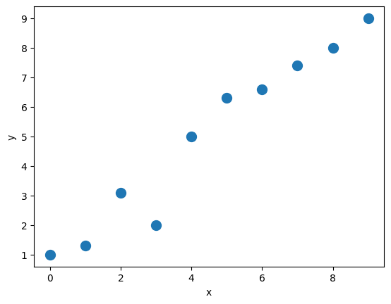

Next, we will standardize the features (mean centering and dividing by the standard deviation) and create a PyTorch Dataset for the training set and a corresponding DataLoader.

Here, we set a batch size of 1 for the DataLoader.

Now, we can define our model for linear regression as $z = wx + b$ . Here, we are going to use the torch.nn module. It provides predefined layers for building complex NN models, but to start, you will learn how to define a model from scratch. Later in this chapter, you will see how to use those predefined layers.

from torch.utils.data import TensorDataset
from torch.utils.data import DataLoader


X_train_norm = (X_train - np.mean(X_train)) / np.std(X_train)
X_train_norm = torch.from_numpy(X_train_norm)

# On some computers the explicit cast to .float() is necessary
y_train = torch.from_numpy(y_train).float()

train_ds = TensorDataset(X_train_norm, y_train)

batch_size = 1
train_dl = DataLoader(train_ds, batch_size, shuffle=True)

For this regression problem, we will define a linear regression model from scratch. We will define the parameters of our model, weight and bias, which correspond to the weight and the bias parameters, respectively. Finally, we will define the model() function to determine how this model uses the input data to generate its output.

torch.manual_seed(1)
weight = torch.randn(1)
weight.requires_grad_()
bias = torch.zeros(1, requires_grad=True)

def model(xb):
    return xb @ weight + bias

After defining the model, we can define the loss function that we want to minimize to find the optimal model weights. Here, we will choose the mean squared error (MSE) as our loss function.

def loss_fn(input, target):
    return (input-target).pow(2).mean()

Furthermore, to learn the weight parameters of the model, we will use stochastic gradient descent (SGD). In this subsection, we will implement this training via the SGD procedure by ourselves, but in the next subsection, we will use the SGD method from the optimization package, torch.optim, to do the same thing.

To implement the SGD algorithm, we need to compute the gradients. Rather than manually computing the gradients, we will use torch.autograd.backward function. We will cover torch.autograd and its different classes and functions in the later chapter.

Now, we can set the learning rate and train the model for 200 epochs. The code for training the model against the batched version of the dataset is as follows.

learning_rate = 0.001
num_epochs = 200
log_epochs = 10

for epoch in range(num_epochs):
    for x_batch, y_batch in train_dl:
        pred = model(x_batch)
        loss = loss_fn(pred, y_batch)
        loss.backward()

        with torch.no_grad():
            weight -= weight.grad * learning_rate
            bias -= bias.grad * learning_rate
            weight.grad.zero_()  # set weights gradients back to zero
            bias.grad.zero_()
 
    if epoch % log_epochs==0:
        print(f'Epoch {epoch}  Loss {loss.item():.4f}')

Epoch 0  Loss 45.0782
Epoch 10  Loss 26.4366
Epoch 20  Loss 1.5918
Epoch 30  Loss 14.1307
Epoch 40  Loss 11.6038
Epoch 50  Loss 6.3084
Epoch 60  Loss 0.6349
Epoch 70  Loss 3.1374
Epoch 80  Loss 1.9999
Epoch 90  Loss 0.3133
Epoch 100  Loss 0.7653
Epoch 110  Loss 1.0039
Epoch 120  Loss 0.0235
Epoch 130  Loss 0.5176
Epoch 140  Loss 0.0759
Epoch 150  Loss 1.8789
Epoch 160  Loss 0.0008
Epoch 170  Loss 0.0866
Epoch 180  Loss 0.0646
Epoch 190  Loss 0.0011

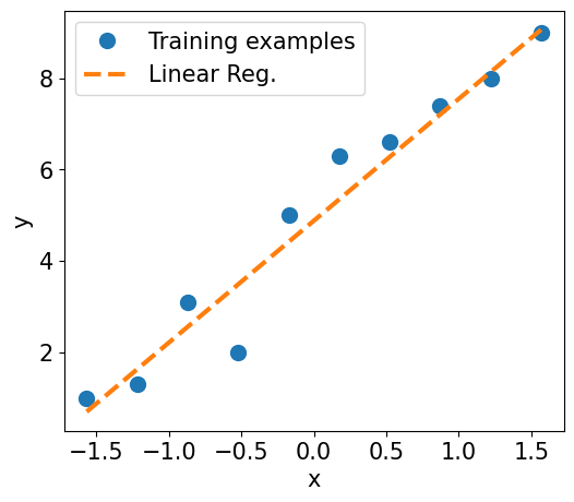
Let’s look at the trained model and plot it. For the test data, we will create a NumPy array of values evenly spaced between 0 and 9. Since we trained our model with standardized features, we will also apply the same standardization to the test data.

print('Final Parameters:', weight.item(), bias.item())
 
X_test = np.linspace(0, 9, num=100, dtype='float32').reshape(-1, 1)
X_test_norm = (X_test - np.mean(X_train)) / np.std(X_train)
X_test_norm = torch.from_numpy(X_test_norm)
y_pred = model(X_test_norm).detach().numpy()


fig = plt.figure(figsize=(13, 5))
ax = fig.add_subplot(1, 2, 1)
plt.plot(X_train_norm, y_train, 'o', markersize=10)
plt.plot(X_test_norm, y_pred, '--', lw=3)
plt.legend(['Training examples', 'Linear Reg.'], fontsize=15)
ax.set_xlabel('x', size=15)
ax.set_ylabel('y', size=15)
ax.tick_params(axis='both', which='major', labelsize=15)
 
#plt.savefig('figures/12_08.pdf')

plt.show()

Final Parameters: 2.6696107387542725 4.879678249359131

12.4.3.Model training via the torch.nn and torch.optim modules¶

In the previous example, we saw how to train a model by writing a custom loss function loss_fn() and applied stochastic gradient descent optimization. However, writing the loss function and gradient updates can be a repeatable task across different projects. The torch.nn module provides a set of loss functions, and torch.optim supports most commonly used optimization algorithms that can be called to update the parameters based on the computed gradients. To see how they work, let’s create a new MSE loss function and a stochastic gradient descent optimizer.

Note that here we use the torch.nn.Linear class for the linear layer instead of manually defining it.

import torch.nn as nn

input_size = 1
output_size = 1
model = nn.Linear(input_size, output_size)

loss_fn = nn.MSELoss(reduction='mean')

optimizer = torch.optim.SGD(model.parameters(), lr=learning_rate)

Now, we can simply call the step() method of the optimizer to train the model. We can pass a batched dataset (such as train_dl, which was created in the previous example).


for epoch in range(num_epochs):
    for x_batch, y_batch in train_dl:
        # 1. Generate predictions
        pred = model(x_batch)[:, 0] 

        # 2. Calculate loss
        loss = loss_fn(pred, y_batch)

        # 3. Compute gradients
        loss.backward()

        # 4. Update parameters using gradients
        optimizer.step()

        # 5. Reset the gradients to zero
        optimizer.zero_grad()
        
    if epoch % log_epochs==0:
        print(f'Epoch {epoch}  Loss {loss.item():.4f}')

Epoch 0  Loss 24.6684
Epoch 10  Loss 29.1377
Epoch 20  Loss 20.9207
Epoch 30  Loss 0.1257
Epoch 40  Loss 12.4922
Epoch 50  Loss 1.7845
Epoch 60  Loss 7.6425
Epoch 70  Loss 2.5606
Epoch 80  Loss 0.0157
Epoch 90  Loss 0.7548
Epoch 100  Loss 0.8412
Epoch 110  Loss 0.4923
Epoch 120  Loss 0.0823
Epoch 130  Loss 0.0794
Epoch 140  Loss 0.0891
Epoch 150  Loss 0.0973
Epoch 160  Loss 0.1043
Epoch 170  Loss 0.1103
Epoch 180  Loss 0.0009
Epoch 190  Loss 0.0764

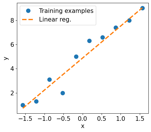
After the model is trained, visualize the results and make sure that they are similar to the results of the previous method. To obtain the weight and bias parameters, we can do the following.

print('Final Parameters:', model.weight.item(), model.bias.item())
 
X_test = np.linspace(0, 9, num=100, dtype='float32').reshape(-1, 1)
X_test_norm = (X_test - np.mean(X_train)) / np.std(X_train)
X_test_norm = torch.from_numpy(X_test_norm)
y_pred = model(X_test_norm).detach().numpy()


fig = plt.figure(figsize=(13, 5))
ax = fig.add_subplot(1, 2, 1)
plt.plot(X_train_norm.detach().numpy(), y_train.detach().numpy(), 'o', markersize=10)
plt.plot(X_test_norm.detach().numpy(), y_pred, '--', lw=3)
plt.legend(['Training examples', 'Linear reg.'], fontsize=15)
ax.set_xlabel('x', size=15)
ax.set_ylabel('y', size=15)
ax.tick_params(axis='both', which='major', labelsize=15)
 
#plt.savefig('ch12-linreg-2.pdf')

plt.show()

Final Parameters: 2.6496422290802 4.87706995010376

12.4.4.Building a multilayer perceptron for classifying flowers in the Iris dataset¶

In the previous example, you saw how to build a model from scratch. We trained this model using stochastic gradient descent optimization. While we started our journey based on the simplest possible example, you can see that defining the model from scratch, even for such a simple case, is neither appealing nor good practice. PyTorch instead provides already defined layers through torch.nn that can be readily used as the building blocks of an NN model. In this section, you will learn how to use these layers to solve a classification task using the Iris flower dataset (identifying between three species of irises) and build a two-layer perceptron using the torch.nn module. First, let’s get the data from sklearn.datasets.

Here, we randomly select 100 samples (2/3) for training and 50 samples (1/3) for testing.

from sklearn.datasets import load_iris
from sklearn.model_selection import train_test_split 

iris = load_iris()
X = iris['data']
y = iris['target']
 
X_train, X_test, y_train, y_test = train_test_split(
    X, y, test_size=1./3, random_state=1)

Next, we standardize the features (mean centering and dividing by the standard deviation) and create a PyTorch Dataset for the training set and a corresponding DataLoader. Here, we set the batch size to 2 for the DataLoader.

from torch.utils.data import TensorDataset
from torch.utils.data import DataLoader

X_train_norm = (X_train - np.mean(X_train)) / np.std(X_train)
X_train_norm = torch.from_numpy(X_train_norm).float()
y_train = torch.from_numpy(y_train) 

train_ds = TensorDataset(X_train_norm, y_train)

torch.manual_seed(1)
batch_size = 2
train_dl = DataLoader(train_ds, batch_size, shuffle=True)

Now, we are ready to use the torch.nn module to build a model efficiently. In particular, using the nn.Module class, we can stack a few layers and build an NN. You can see the list of all the layers that are already available at https://pytorch.org/docs/stable/nn.html.

For this problem, we are going to use the Linear layer, which is also known as a fully connected layer or dense layer, and can be best represented by $f(w \times x+b)$ .

$x$ : a tensor containing the input features
$w$ and $b$ : the weight matrix and the bias vector
$f$ : the activation function

Each layer in an NN receives its inputs from the preceding layer; therefore, its dimensionality (rank and shape) is fixed. Typically, we need to concern ourselves with the dimensionality of output only when we design an NN architecture. Here, we want to define a model with two hidden layers.

The first layer receives an input of four features and projects them to 16 neurons.
The second layer receives the output of the previous layer (which has a size of 16) and projects them to three output neurons, since we have three class labels.

Here, we used the sigmoid activation function for the first layer and softmax activation for the last (output) layer. Softmax activation in the last layer is used to support multiclass classification since we have three class labels here (which is why we have three neurons in the output layer).

class Model(nn.Module):
    def __init__(self, input_size, hidden_size, output_size):
        super().__init__()
        self.layer1 = nn.Linear(input_size, hidden_size)  
        self.layer2 = nn.Linear(hidden_size, output_size)  

    def forward(self, x):
        x = self.layer1(x)
        x = nn.Sigmoid()(x)
        x = self.layer2(x)
        x = nn.Softmax(dim=1)(x)
        return x
    
input_size = X_train_norm.shape[1]
hidden_size = 16
output_size = 3
 
model = Model(input_size, hidden_size, output_size)

Next, we specify the loss function as cross-entropy loss and the optimizer as Adam.

learning_rate = 0.001

loss_fn = nn.CrossEntropyLoss()
 
optimizer = torch.optim.Adam(model.parameters(), lr=learning_rate)

Now, we can train the model. We will specify the number of epochs to be 100. The loss_hist and accuracy_hist lists keep the training loss and the training accuracy after each epoch.

num_epochs = 100
loss_hist = [0] * num_epochs
accuracy_hist = [0] * num_epochs

for epoch in range(num_epochs):

    for x_batch, y_batch in train_dl:
        pred = model(x_batch)
        loss = loss_fn(pred, y_batch.long())
        loss.backward()
        optimizer.step()
        optimizer.zero_grad()
    
        loss_hist[epoch] += loss.item()*y_batch.size(0)
        is_correct = (torch.argmax(pred, dim=1) == y_batch).float()
        accuracy_hist[epoch] += is_correct.sum()
        
    loss_hist[epoch] /= len(train_dl.dataset)
    accuracy_hist[epoch] /= len(train_dl.dataset)

We can use this to visualize the learning curves as follows.

fig = plt.figure(figsize=(12, 5))
ax = fig.add_subplot(1, 2, 1)
ax.plot(loss_hist, lw=3)
ax.set_title('Training loss', size=15)
ax.set_xlabel('Epoch', size=15)
ax.tick_params(axis='both', which='major', labelsize=15)

ax = fig.add_subplot(1, 2, 2)
ax.plot(accuracy_hist, lw=3)
ax.set_title('Training accuracy', size=15)
ax.set_xlabel('Epoch', size=15)
ax.tick_params(axis='both', which='major', labelsize=15)
plt.tight_layout()

#plt.savefig('figures/12_09.pdf')
 
plt.show()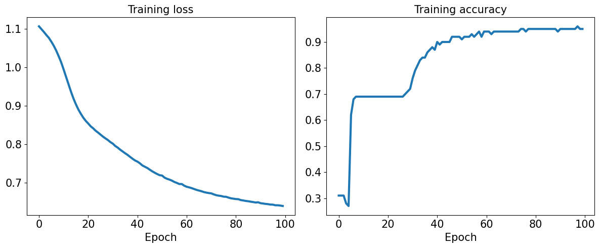

12.4.5.Evaluating the trained model on the test dataset¶

We can now evaluate the classification accuracy of the trained model on the test dataset. Since we trained our model with standardized features, we also applied the same standardization to the test data. The classification accuracy is 0.98 (that is, 98 percent).

X_test_norm = (X_test - np.mean(X_train)) / np.std(X_train)
X_test_norm = torch.from_numpy(X_test_norm).float()
y_test = torch.from_numpy(y_test) 
pred_test = model(X_test_norm)

correct = (torch.argmax(pred_test, dim=1) == y_test).float()
accuracy = correct.mean()
 
print(f'Test Acc.: {accuracy:.4f}')

Test Acc.: 0.9800

12.4.6.Saving and reloading the trained model¶

Trained models can be saved on disk for future use. Calling save(model) will save both the model architecture and all the learned parameters. As a common convention, we can save models using a 'pt' or 'pth' file extension.

path = 'iris_classifier.pt'
torch.save(model, path)

Now, let’s reload the saved model. Since we have saved both the model architecture and the weights, we can easily rebuild and reload the parameters in just one line.

model_new = torch.load(path)

Try to verify the model architecture by calling model_new.eval().

model_new.eval()

Model(
  (layer1): Linear(in_features=4, out_features=16, bias=True)
  (layer2): Linear(in_features=16, out_features=3, bias=True)
)

Finally, let’s evaluate this new model that is reloaded on the test dataset to verify that the results are the same as before.

pred_test = model_new(X_test_norm)

correct = (torch.argmax(pred_test, dim=1) == y_test).float()
accuracy = correct.mean()
 
print(f'Test Acc.: {accuracy:.4f}')

Test Acc.: 0.9800

If you want to save only the learned parameters, you can use save(model.state_dict()) as follows.

path = 'iris_classifier_state.pt'
torch.save(model.state_dict(), path)

To reload the saved parameters, we first need to construct the model as we did before, then feed the loaded parameters to the model.

model_new = Model(input_size, hidden_size, output_size)
model_new.load_state_dict(torch.load(path))

<All keys matched successfully>

12.5.Choosing activation functions for multilayer neural networks¶

The logistic (sigmoid) activation function probably mimics the concept of a neuron in a brain most closely - we can think of it as the probability of whether a neuron fires. However, the logistic (sigmoid) activation function can be problematic if we have highly negative input, since the output of the sigmoid function will be close to zero in this case. If the sigmoid function returns output that is close to zero, the NN will learn very slowly, and it will be more likely to get trapped in the local minima of the loss landscape during training. This is why people often prefer a hyperbolic tangent as an activation function in hidden layers.

Before we discuss what a hyperbolic tangent looks like, let’s briefly recapitulate some of the basics of the logistic function and look at a generalization that makes it more useful for multiclass classification problems.

12.5.1.Logistic function recap¶

Recall that the logistic function is a special case of a sigmoid function.

We can use a logistic function to model the probability that sample $x$ belongs to the positive class (class 1) in a binary classification task.

The given net input, $z$ :
$z=w_0 x_0+w_1 x_1+\cdots+w_m x_m=\sum_{i=0}^m w_i x_i=w^{\mathrm{T}} x$
(1)
The logistic (sigmoid) function:
$\sigma_{\text {logistic }}(z)=\frac{1}{1+e^{-z}}$
(2)
Note that $w_0$ is the bias unit ( $y$ -axis intercept, which means $x_0=1$ ).

To provide a more concrete example, let’s take a model for a two-dimensional data point, $x$ , and a model with the following weight coefficients assigned to the $w$ vector.

Result explanation

If we calculate the net input $(z)$ and use it to activate a logistic neuron with those particular feature values and weight coefficients, we get a value of 0.888 , which we can interpret as an 88.8 percent probability that this particular sample, $x$ , belongs to the positive class.

import numpy as np

X = np.array([1, 1.4, 2.5]) ## first value must be 1
w = np.array([0.4, 0.3, 0.5])

def net_input(X, w):
    return np.dot(X, w)

def logistic(z):
    return 1.0 / (1.0 + np.exp(-z))

def logistic_activation(X, w):
    z = net_input(X, w)
    return logistic(z)

print(f'P(y=1|x) = {logistic_activation(X, w):.3f}')

P(y=1|x) = 0.888

The following code example, an output layer consisting of multiple logistic activation units does not produce meaningful, interpretable probability values since we are not using one-hot encoding.

Result explanation

As you can see in the output, the resulting values cannot be interpreted as probabilities for a three-class problem. The reason for this is that they do not sum to 1. However, this is, in fact, not a big concern if we use our model to predict only the class labels and not the class membership probabilities.

# W : array with shape = (n_output_units, n_hidden_units+1)
# Note that the first column are the bias units
W = np.array([[1.1, 1.2, 0.8, 0.4],
              [0.2, 0.4, 1.0, 0.2],
              [0.6, 1.5, 1.2, 0.7]])


# A : data array with shape = (n_hidden_units + 1, n_samples)
# Note that the first column of this array must be 1
A = np.array([[1, 0.1, 0.4, 0.6]])
Z = np.dot(W, A[0])
y_probas = logistic(Z)
print('Net Input: \n', Z)

print('Output Units:\n', y_probas)

Net Input: 
 [1.78 0.76 1.65]
Output Units:
 [0.85569687 0.68135373 0.83889105]

One way to predict the class label from the output units obtained earlier is to use the maximum value. In certain contexts, it can be useful to compute meaningful class probabilities for multiclass predictions.

In the next section, we will take a look at a generalization of the logistic function, the softmax function, which can help us with this task.

y_class = np.argmax(Z, axis=0)
print('Predicted class label:', y_class)

Predicted class label: 0

12.5.2.Estimating class probabilities in multiclass classification via the softmax function¶

The softmax function is a soft form of the argmax function; instead of giving a single class index, it provides the probability of each class. Therefore, it allows us to compute meaningful class probabilities in multiclass settings (multinomial logistic regression).

In softmax, the probability of a particular sample with net input $z$ belonging to the $i$ th class can be computed with a normalization term in the denominator, that is, the sum of the exponentially weighted linear functions:

p(z)=\sigma(z)=\frac{e^{z_i}}{\sum_{j=1}^M e^{z_j}}

(3)

Result explanation

As you can see, the predicted class probabilities now sum to 1, as we would expect. It is also notable that the predicted class label is the same as when we applied the argmax function to the logistic output.

def softmax(z):
    return np.exp(z) / np.sum(np.exp(z))

y_probas = softmax(Z)
print('Probabilities:\n', y_probas)

print('\nSum up the output probabilities: ', np.sum(y_probas))

Probabilities:
 [0.44668973 0.16107406 0.39223621]

Sum up the output probabilities:  1.0

It may help to think of the result of the softmax function as a normalized output that is useful for obtaining meaningful class-membership predictions in multiclass settings. Therefore, when we build a multiclass classification model in PyTorch, we can use the torch. softmax() function to estimate the probabilities of each class membership for an input batch of examples.

To see how we can use the torch.softmax() activation function in PyTorch, we will convert z to a tensor in the following code, with an additional dimension reserved for the batch size.

torch.softmax(torch.from_numpy(Z), dim=0)

tensor([0.4467, 0.1611, 0.3922], dtype=torch.float64)

12.5.3.Broadening the output spectrum using a hyperbolic tangent¶

import matplotlib.pyplot as plt
%matplotlib inline

def tanh(z):
    e_p = np.exp(z)
    e_m = np.exp(-z)
    return (e_p - e_m) / (e_p + e_m)

z = np.arange(-5, 5, 0.005)
log_act = logistic(z)
tanh_act = tanh(z)
plt.ylim([-1.5, 1.5])
plt.xlabel('Net input $z$')
plt.ylabel('Activation $\phi(z)$')
plt.axhline(1, color='black', linestyle=':')
plt.axhline(0.5, color='black', linestyle=':')
plt.axhline(0, color='black', linestyle=':')
plt.axhline(-0.5, color='black', linestyle=':')
plt.axhline(-1, color='black', linestyle=':')
plt.plot(z, tanh_act,
    linewidth=3, linestyle='--',
    label='Tanh')
plt.plot(z, log_act,
    linewidth=3,
    label='Logistic')
plt.legend(loc='lower right')
plt.tight_layout()

#plt.savefig('figures/12_10.pdf')
plt.show()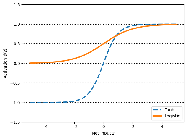

print('tanh in Numpy:\n', np.tanh(z))
print('\ntanh in PyTorch:\n', torch.tanh(torch.from_numpy(z)))

tanh in Numpy:
 [-0.9999092  -0.99990829 -0.99990737 ...  0.99990644  0.99990737
  0.99990829]

tanh in PyTorch:
 tensor([-0.9999, -0.9999, -0.9999,  ...,  0.9999,  0.9999,  0.9999],
       dtype=torch.float64)

from scipy.special import expit

print('logistic in SciPy:\n', expit(z))
print('\nlogistic in PyTorch:\n', torch.sigmoid(torch.from_numpy(z)))

logistic in SciPy:
 [0.00669285 0.00672617 0.00675966 ... 0.99320669 0.99324034 0.99327383]

logistic in PyTorch:
 tensor([0.0067, 0.0067, 0.0068,  ..., 0.9932, 0.9932, 0.9933],
       dtype=torch.float64)

12.5.4.Rectified linear unit activation¶

The rectified linear unit (ReLU) is another activation function that is often used in deep NNs.

Vanishing gradient problem in tanh and logistic activations

To understand this problem, let’s assume that we initially have the net input $z_1=20$ , which changes to $z_2=25$ . Computing the tanh activation, we get $\sigma\left(z_1\right)=1.0$ and $\sigma\left(z_2\right)=1.0$ , which shows no change in the output (due to the asymptotic behavior of the tanh function and numerical errors). This means that the derivative of activations with respect to the net input diminishes as $z$ becomes large. As a result, learning the weights during the training phase becomes very slow because the gradient terms may be very close to zero.

Vanishing gradient solution: ReLU

ReLU activation addresses this issue. Mathematically, ReLU is defined as follows:

\sigma(z)=\max (0, z)

(4)

ReLU is still a nonlinear function that is good for learning complex functions with NNs. Besides this, the derivative of ReLU, with respect to its input, is always 1 for positive input values. Therefore, it solves the problem of vanishing gradients, making it suitable for deep NNs.

torch.relu(torch.from_numpy(z))

tensor([0.0000, 0.0000, 0.0000,  ..., 4.9850, 4.9900, 4.9950],
       dtype=torch.float64)

Summary¶

IPythonImage(filename='figures/12_11.png', width=500)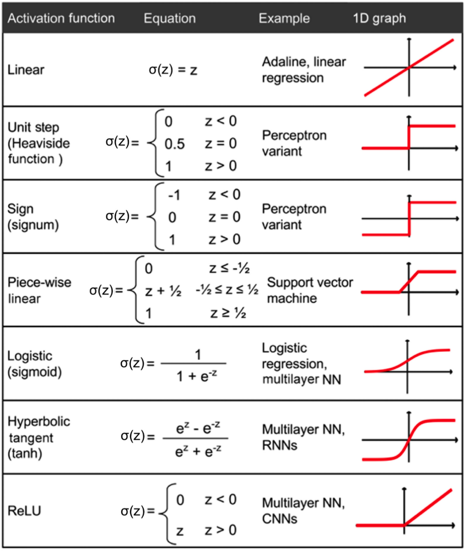

Readers may ignore the next cell.

! python ../.convert_notebook_to_script.py --input ch12_part2.ipynb --output ch12_part2.py

[NbConvertApp] Converting notebook ch12_part2.ipynb to script
[NbConvertApp] Writing 12165 bytes to ch12_part2.py