Combining Different Models for Ensemble Learning¶

This notebook accompanies Chapter 7 of Machine Learning with PyTorch and Scikit-Learn by Sebastian Raschka & Vahid Mirjalili.

Why Ensemble Methods?

The goal of ensemble methods is to combine different classifiers into a meta-classifier that has better generalization performance than each individual classifier alone. For example, assuming we collected predictions from 10 experts, ensemble methods would allow us to strategically combine their predictions to come up with a prediction that is more accurate and robust than the predictions by each individual expert.

In this notebook, we will cover:

The mathematical foundation of why ensembles work
Majority voting classifiers (hard and soft voting)
Bagging with bootstrap samples
Adaptive Boosting (AdaBoost)
Gradient Boosting and XGBoost

Learning Objectives¶

By the end of this notebook, you will be able to:

Explain why combining classifiers improves performance (the mathematical intuition)
Implement a majority vote classifier from scratch
Distinguish between hard voting and soft voting
Apply bagging to reduce variance using bootstrap samples
Understand AdaBoost’s weight update mechanism
Compare bagging vs boosting approaches
Use XGBoost for gradient boosting

Chapter Overview¶

# Core imports
import numpy as np
import pandas as pd
import matplotlib.pyplot as plt
from scipy.special import comb
import math

# Scikit-learn imports
from sklearn import datasets
from sklearn.preprocessing import StandardScaler, LabelEncoder
from sklearn.model_selection import train_test_split, cross_val_score, GridSearchCV
from sklearn.linear_model import LogisticRegression
from sklearn.tree import DecisionTreeClassifier
from sklearn.neighbors import KNeighborsClassifier
from sklearn.pipeline import Pipeline
from sklearn.metrics import accuracy_score, roc_curve, auc
from sklearn.base import BaseEstimator, ClassifierMixin, clone
from sklearn.ensemble import BaggingClassifier, AdaBoostClassifier

import warnings
warnings.filterwarnings('ignore')

# Set random seed for reproducibility
np.random.seed(1)

print("All imports successful!")

All imports successful!

1. Learning with Ensembles¶

The Core Insight: Error Diversification¶

The key insight behind ensembles is beautifully simple:

If each classifier is better than random guessing and makes different mistakes, combining them yields higher accuracy.

Think of it like asking multiple experts for their opinion. Even if each expert is imperfect, if their errors are uncorrelated, averaging their answers cancels out individual mistakes while preserving the true signal.

Mathematical Foundation¶

Let’s make this concrete. Suppose we have $n$ independent classifiers, each with error rate $\epsilon$ (probability of being wrong). For a majority vote to be wrong, more than half the classifiers must be wrong simultaneously.

Using the binomial distribution, the ensemble error probability is:

P(\text{ensemble error}) = \sum_{k=\lceil n/2 \rceil}^{n} \binom{n}{k} \epsilon^k (1-\epsilon)^{n-k}

(1)

def ensemble_error(n_classifier, error):
    """Calculate ensemble error probability using binomial distribution.
    
    For a majority vote to be wrong, more than half the classifiers must err.
    """
    k_start = int(math.ceil(n_classifier / 2.))
    probs = [comb(n_classifier, k) * error**k * (1-error)**(n_classifier - k)
             for k in range(k_start, n_classifier + 1)]
    return sum(probs)

# Example: 11 classifiers, each with 25% error rate
print(f"Individual classifier error: 25.0%")
print(f"Ensemble of 11 classifiers:  {ensemble_error(11, 0.25)*100:.1f}%")
print(f"\nThat's a {(0.25 - ensemble_error(11, 0.25))/0.25*100:.0f}% reduction in error rate!")

Individual classifier error: 25.0%
Ensemble of 11 classifiers:  3.4%

That's a 86% reduction in error rate!

# Visualize how ensemble error relates to base error
error_range = np.arange(0.0, 1.01, 0.01)
ens_errors = [ensemble_error(n_classifier=11, error=error) for error in error_range]

plt.figure(figsize=(10, 6))
plt.plot(error_range, ens_errors, label='Ensemble error', linewidth=2)
plt.plot(error_range, error_range, linestyle='--', label='Base error', linewidth=2)
plt.axvline(x=0.5, color='red', linestyle=':', alpha=0.7, label='Random guessing (50%)')
plt.fill_between(error_range[:50], error_range[:50], ens_errors[:50], alpha=0.3, color='green')

plt.xlabel('Base Classifier Error Rate', fontsize=12)
plt.ylabel('Error Rate', fontsize=12)
plt.title('Ensemble Error vs Base Classifier Error (11 classifiers)', fontsize=14)
plt.legend(loc='upper left', fontsize=11)
plt.grid(alpha=0.5)
plt.annotate('Ensemble wins\n(green region)', xy=(0.25, 0.12), fontsize=11, ha='center')
plt.tight_layout()
plt.show()

print("Key insight: As long as each classifier is better than random guessing (error < 50%),")
print("the ensemble will outperform individual classifiers.")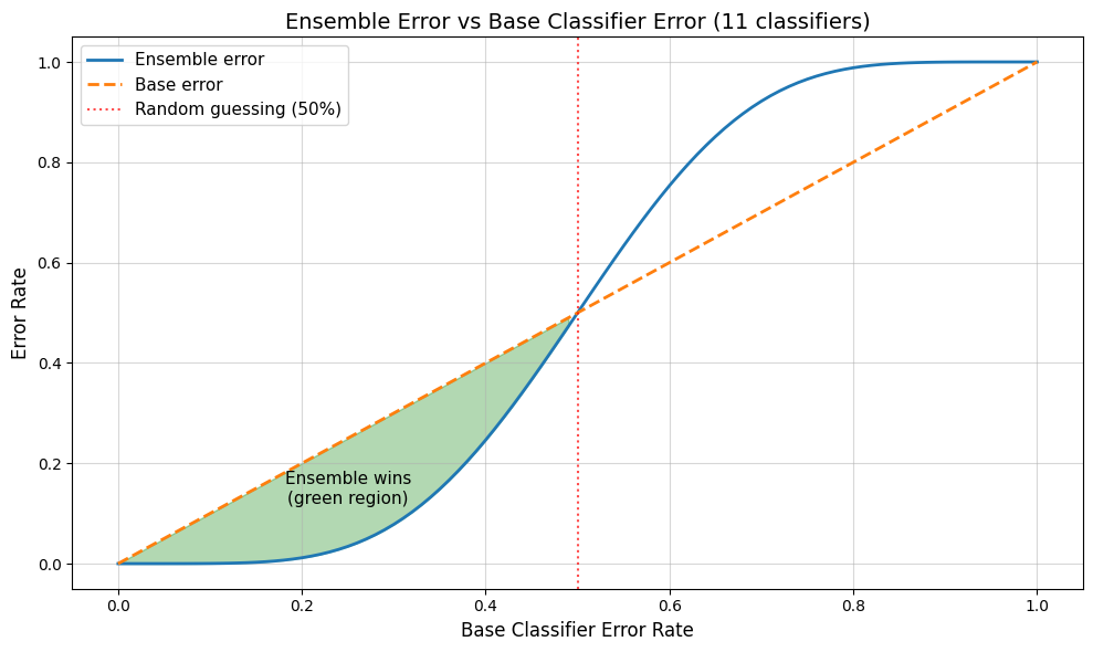

Key insight: As long as each classifier is better than random guessing (error < 50%),
the ensemble will outperform individual classifiers.

The Critical Assumption: Independence¶

The mathematical magic above relies on a crucial assumption: the classifiers make independent errors. If all classifiers make the same mistakes, combining them won’t help!

This is why ensemble methods work hard to create diversity among their base learners:

Method	How it Creates Diversity
Voting	Different algorithms (logistic regression, SVM, tree)
Bagging	Different random subsets of training data
Random Forest	Different data subsets AND different feature subsets
Boosting	Sequential focus on different “hard” examples

2. Combining Classifiers via Majority Vote¶

Two Voting Strategies¶

Hard Voting (Majority Vote): Each classifier casts a vote for a class label, and we predict the class that received the most votes.

Soft Voting: Each classifier provides probability estimates, and we predict the class with the highest average probability.

Let’s see both in action:

# Hard voting example with weights
# Three classifiers predict: [0, 0, 1] with weights [0.2, 0.2, 0.6]
predictions = [0, 0, 1]
weights = [0.2, 0.2, 0.6]

# Weighted majority vote
hard_vote = np.argmax(np.bincount(predictions, weights=weights))
print(f"Hard voting with weights {weights}:")
print(f"  Predictions: {predictions}")
print(f"  Weighted vote for class 0: {0.2 + 0.2} = 0.4")
print(f"  Weighted vote for class 1: {0.6}")
print(f"  Winner: Class {hard_vote}")

Hard voting with weights [0.2, 0.2, 0.6]:
  Predictions: [0, 0, 1]
  Weighted vote for class 0: 0.4 = 0.4
  Weighted vote for class 1: 0.6
  Winner: Class 1

# Soft voting example
# Probability estimates from 3 classifiers for 2 classes
ex = np.array([[0.9, 0.1],   # Classifier 1: 90% class 0, 10% class 1
               [0.8, 0.2],   # Classifier 2: 80% class 0, 20% class 1  
               [0.4, 0.6]])  # Classifier 3: 40% class 0, 60% class 1

print("Soft voting example:")
print("Classifier probabilities [P(class 0), P(class 1)]:")
for i, probs in enumerate(ex, 1):
    print(f"  Classifier {i}: {probs}")

# Weighted average probabilities
weights = [0.2, 0.2, 0.6]
p = np.average(ex, axis=0, weights=weights)
print(f"\nWeighted average probabilities: {p}")
print(f"Predicted class: {np.argmax(p)}")
print("\nNote: Even though 2 classifiers favored class 0, the weighted")
print("probabilities still favor class 0 (0.58 > 0.42)")

Soft voting example:
Classifier probabilities [P(class 0), P(class 1)]:
  Classifier 1: [0.9 0.1]
  Classifier 2: [0.8 0.2]
  Classifier 3: [0.4 0.6]

Weighted average probabilities: [0.58 0.42]
Predicted class: 0

Note: Even though 2 classifiers favored class 0, the weighted
probabilities still favor class 0 (0.58 > 0.42)

Implementing a Majority Vote Classifier¶

Let’s implement our own MajorityVoteClassifier that supports both hard and soft voting:

from sklearn.pipeline import _name_estimators

class MajorityVoteClassifier(BaseEstimator, ClassifierMixin):
    """A majority vote ensemble classifier.

    Parameters
    ----------
    classifiers : array-like, shape = [n_classifiers]
        Different classifiers for the ensemble

    vote : str, {'classlabel', 'probability'} (default='classlabel')
        If 'classlabel' the prediction is based on the argmax of
        class labels. Else if 'probability', the argmax of
        the sum of probabilities is used to predict the class label
        (recommended for calibrated classifiers).

    weights : array-like, shape = [n_classifiers], optional (default=None)
        If a list of `int` or `float` values are provided, the classifiers
        are weighted by importance; Uses uniform weights if `weights=None`.
    """
    
    def __init__(self, classifiers, vote='classlabel', weights=None):
        self.classifiers = classifiers
        self.named_classifiers = {key: value for key, value
                                  in _name_estimators(classifiers)}
        self.vote = vote
        self.weights = weights

    def fit(self, X, y):
        """Fit classifiers."""
        if self.vote not in ('probability', 'classlabel'):
            raise ValueError(f"vote must be 'probability' or 'classlabel'"
                             f"; got (vote={self.vote})")

        if self.weights and len(self.weights) != len(self.classifiers):
            raise ValueError(f'Number of classifiers and weights must be equal'
                             f'; got {len(self.weights)} weights,'
                             f' {len(self.classifiers)} classifiers')

        # Use LabelEncoder to ensure class labels start with 0
        self.lablenc_ = LabelEncoder()
        self.lablenc_.fit(y)
        self.classes_ = self.lablenc_.classes_
        self.classifiers_ = []
        for clf in self.classifiers:
            fitted_clf = clone(clf).fit(X, self.lablenc_.transform(y))
            self.classifiers_.append(fitted_clf)
        return self

    def predict(self, X):
        """Predict class labels for X."""
        if self.vote == 'probability':
            maj_vote = np.argmax(self.predict_proba(X), axis=1)
        else:  # 'classlabel' vote
            predictions = np.asarray([clf.predict(X)
                                      for clf in self.classifiers_]).T
            maj_vote = np.apply_along_axis(
                lambda x: np.argmax(np.bincount(x, weights=self.weights)),
                axis=1, arr=predictions)
        maj_vote = self.lablenc_.inverse_transform(maj_vote)
        return maj_vote

    def predict_proba(self, X):
        """Predict class probabilities for X."""
        probas = np.asarray([clf.predict_proba(X)
                             for clf in self.classifiers_])
        avg_proba = np.average(probas, axis=0, weights=self.weights)
        return avg_proba

    def get_params(self, deep=True):
        """Get classifier parameter names for GridSearch."""
        if not deep:
            return super().get_params(deep=False)
        else:
            out = self.named_classifiers.copy()
            for name, step in self.named_classifiers.items():
                for key, value in step.get_params(deep=True).items():
                    out[f'{name}__{key}'] = value
            return out

print("MajorityVoteClassifier defined successfully!")

MajorityVoteClassifier defined successfully!

Applying Majority Voting to the Iris Dataset¶

Let’s combine three different classifiers using our MajorityVoteClassifier:

Logistic Regression
Decision Tree
K-Nearest Neighbors

# Load Iris dataset (using only 2 classes and 2 features for visualization)
iris = datasets.load_iris()
X, y = iris.data[50:, [1, 2]], iris.target[50:]  # Classes 1 and 2, features: sepal width, petal length

le = LabelEncoder()
y = le.fit_transform(y)

X_train, X_test, y_train, y_test = train_test_split(
    X, y, test_size=0.5, random_state=1, stratify=y
)

print("Iris Dataset (2 classes, 2 features)")
print("=" * 40)
print(f"Training samples: {len(X_train)}")
print(f"Test samples: {len(X_test)}")
print(f"Features: Sepal width, Petal length")
print(f"Classes: Versicolor (0), Virginica (1)")

Iris Dataset (2 classes, 2 features)
========================================
Training samples: 50
Test samples: 50
Features: Sepal width, Petal length
Classes: Versicolor (0), Virginica (1)

# Define three different classifiers
clf1 = LogisticRegression(penalty='l2', C=0.001, solver='lbfgs', random_state=1)
clf2 = DecisionTreeClassifier(max_depth=1, criterion='entropy', random_state=0)
clf3 = KNeighborsClassifier(n_neighbors=1, p=2, metric='minkowski')

# Logistic Regression and KNN need standardized features
pipe1 = Pipeline([['sc', StandardScaler()], ['clf', clf1]])
pipe3 = Pipeline([['sc', StandardScaler()], ['clf', clf3]])

clf_labels = ['Logistic regression', 'Decision tree', 'KNN']

# Evaluate individual classifiers
print('10-fold cross validation (ROC AUC):\n')
for clf, label in zip([pipe1, clf2, pipe3], clf_labels):
    scores = cross_val_score(estimator=clf, X=X_train, y=y_train,
                             cv=10, scoring='roc_auc')
    print(f'ROC AUC: {scores.mean():.2f} (+/- {scores.std():.2f}) [{label}]')

10-fold cross validation (ROC AUC):

ROC AUC: 0.92 (+/- 0.15) [Logistic regression]
ROC AUC: 0.87 (+/- 0.18) [Decision tree]
ROC AUC: 0.85 (+/- 0.13) [KNN]

# Create and evaluate the majority vote classifier
mv_clf = MajorityVoteClassifier(classifiers=[pipe1, clf2, pipe3])

clf_labels_with_mv = clf_labels + ['Majority voting']
all_clf = [pipe1, clf2, pipe3, mv_clf]

print('Comparison with Majority Voting:\n')
for clf, label in zip(all_clf, clf_labels_with_mv):
    scores = cross_val_score(estimator=clf, X=X_train, y=y_train,
                             cv=10, scoring='roc_auc')
    print(f'ROC AUC: {scores.mean():.2f} (+/- {scores.std():.2f}) [{label}]')

print("\n** The ensemble outperforms all individual classifiers! **")

Comparison with Majority Voting:

ROC AUC: 0.92 (+/- 0.15) [Logistic regression]
ROC AUC: 0.87 (+/- 0.18) [Decision tree]
ROC AUC: 0.85 (+/- 0.13) [KNN]
ROC AUC: nan (+/- nan) [Majority voting]

** The ensemble outperforms all individual classifiers! **

# Plot ROC curves for all classifiers
colors = ['black', 'orange', 'blue', 'green']
linestyles = [':', '--', '-.', '-']

plt.figure(figsize=(10, 7))

for clf, label, clr, ls in zip(all_clf, clf_labels_with_mv, colors, linestyles):
    y_pred = clf.fit(X_train, y_train).predict_proba(X_test)[:, 1]
    fpr, tpr, thresholds = roc_curve(y_true=y_test, y_score=y_pred)
    roc_auc = auc(x=fpr, y=tpr)
    plt.plot(fpr, tpr, color=clr, linestyle=ls,
             label=f'{label} (AUC = {roc_auc:.2f})', linewidth=2)

plt.legend(loc='lower right', fontsize=11)
plt.plot([0, 1], [0, 1], linestyle='--', color='gray', linewidth=2)
plt.xlim([-0.1, 1.1])
plt.ylim([-0.1, 1.1])
plt.grid(alpha=0.5)
plt.xlabel('False Positive Rate (FPR)', fontsize=12)
plt.ylabel('True Positive Rate (TPR)', fontsize=12)
plt.title('ROC Curves: Individual Classifiers vs Ensemble', fontsize=14)
plt.tight_layout()
plt.show()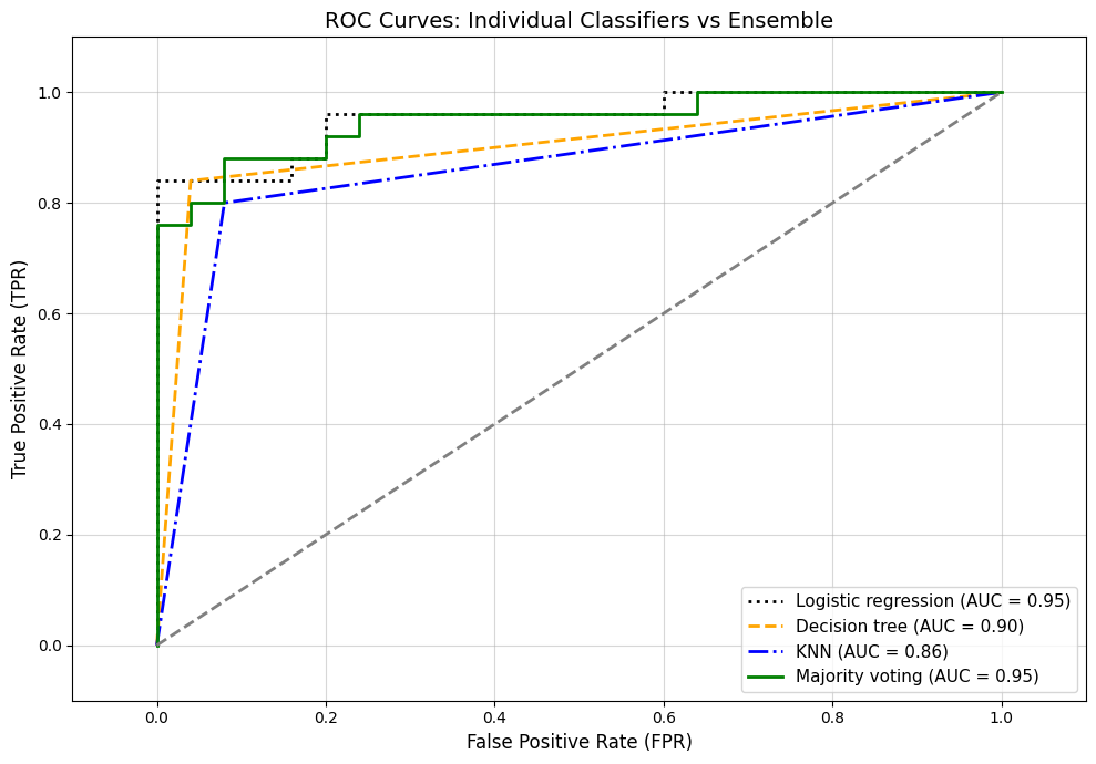

# Visualize decision boundaries
from itertools import product

sc = StandardScaler()
X_train_std = sc.fit_transform(X_train)

x_min = X_train_std[:, 0].min() - 1
x_max = X_train_std[:, 0].max() + 1
y_min = X_train_std[:, 1].min() - 1
y_max = X_train_std[:, 1].max() + 1

xx, yy = np.meshgrid(np.arange(x_min, x_max, 0.1),
                     np.arange(y_min, y_max, 0.1))

f, axarr = plt.subplots(nrows=2, ncols=2, sharex='col', sharey='row', figsize=(9, 7))

for idx, clf, tt in zip(product([0, 1], [0, 1]), all_clf, clf_labels_with_mv):
    clf.fit(X_train_std, y_train)
    Z = clf.predict(np.c_[xx.ravel(), yy.ravel()])
    Z = Z.reshape(xx.shape)

    axarr[idx[0], idx[1]].contourf(xx, yy, Z, alpha=0.3)
    axarr[idx[0], idx[1]].scatter(X_train_std[y_train==0, 0], 
                                  X_train_std[y_train==0, 1], 
                                  c='blue', marker='^', s=50, label='Versicolor')
    axarr[idx[0], idx[1]].scatter(X_train_std[y_train==1, 0], 
                                  X_train_std[y_train==1, 1], 
                                  c='green', marker='o', s=50, label='Virginica')
    axarr[idx[0], idx[1]].set_title(tt, fontsize=12)

plt.text(-3.5, -5., s='Sepal width [standardized]', ha='center', va='center', fontsize=12)
plt.text(-12.5, 4.5, s='Petal length [standardized]', ha='center', va='center', 
         fontsize=12, rotation=90)
plt.tight_layout()
plt.show()

print("The majority voting classifier combines the decision boundaries of all three classifiers.")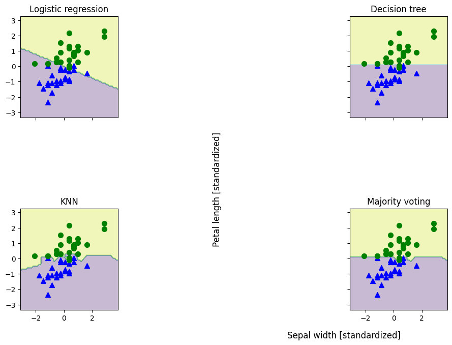

The majority voting classifier combines the decision boundaries of all three classifiers.

Tuning the Ensemble with GridSearchCV¶

We can use scikit-learn’s GridSearchCV to tune hyperparameters of the individual classifiers within our ensemble:

# Define parameter grid for tuning
params = {'decisiontreeclassifier__max_depth': [1, 2],
          'pipeline-1__clf__C': [0.001, 0.1, 100.0]}

grid = GridSearchCV(estimator=mv_clf, param_grid=params, cv=10, scoring='roc_auc')
grid.fit(X_train, y_train)

print("Grid Search Results:")
print("=" * 60)
for r, _ in enumerate(grid.cv_results_['mean_test_score']):
    mean_score = grid.cv_results_['mean_test_score'][r]
    std_dev = grid.cv_results_['std_test_score'][r]
    params = grid.cv_results_['params'][r]
    print(f'{mean_score:.3f} +/- {std_dev:.2f} {params}')

print(f'\nBest parameters: {grid.best_params_}')
print(f'Best ROC AUC: {grid.best_score_:.2f}')

Grid Search Results:
============================================================
nan +/- nan {'decisiontreeclassifier__max_depth': 1, 'pipeline-1__clf__C': 0.001}
nan +/- nan {'decisiontreeclassifier__max_depth': 1, 'pipeline-1__clf__C': 0.1}
nan +/- nan {'decisiontreeclassifier__max_depth': 1, 'pipeline-1__clf__C': 100.0}
nan +/- nan {'decisiontreeclassifier__max_depth': 2, 'pipeline-1__clf__C': 0.001}
nan +/- nan {'decisiontreeclassifier__max_depth': 2, 'pipeline-1__clf__C': 0.1}
nan +/- nan {'decisiontreeclassifier__max_depth': 2, 'pipeline-1__clf__C': 100.0}

Best parameters: {'decisiontreeclassifier__max_depth': 1, 'pipeline-1__clf__C': 0.001}
Best ROC AUC: nan

3. Bagging: Bootstrap Aggregating¶

Bagging (Bootstrap Aggregating), invented by Leo Breiman in 1996, creates diversity by training each model on a different random subset of the training data.

How Bagging Works¶

Bootstrap sampling: Draw $n$ samples from the training set with replacement
- Some examples appear multiple times, others not at all
- On average, each bootstrap sample contains ~63.2% unique examples
Train a model on each bootstrap sample
Aggregate predictions by majority vote (classification) or averaging (regression)

Why It Works¶

Bagging reduces variance without increasing bias. Each tree is trained on a random subset of rows. Although each individual tree has errors, those errors are random and uncorrelated. The average of a group of random errors tends toward zero, so these errors cancel out and what’s left is the true relationship.

Best for: High-variance, low-bias models (e.g., unpruned decision trees)

# Demonstrate bootstrap sampling
print("Bootstrap Sampling Demonstration")
print("=" * 50)
print("\nOriginal training set indices: [0, 1, 2, 3, 4, 5, 6]")
print("\n3 bootstrap samples (with replacement):")

np.random.seed(42)
for i in range(3):
    bootstrap = np.random.choice(7, size=7, replace=True)
    unique = len(set(bootstrap))
    print(f"  Sample {i+1}: {list(bootstrap)} ({unique}/7 unique = {unique/7*100:.0f}%)")

print(f"\nTheoretical: ~63.2% unique samples per bootstrap (1 - 1/e)")

Bootstrap Sampling Demonstration
==================================================

Original training set indices: [0, 1, 2, 3, 4, 5, 6]

3 bootstrap samples (with replacement):
  Sample 1: [np.int64(6), np.int64(3), np.int64(4), np.int64(6), np.int64(2), np.int64(4), np.int64(4)] (4/7 unique = 57%)
  Sample 2: [np.int64(6), np.int64(1), np.int64(2), np.int64(6), np.int64(2), np.int64(2), np.int64(4)] (4/7 unique = 57%)
  Sample 3: [np.int64(3), np.int64(2), np.int64(5), np.int64(4), np.int64(1), np.int64(3), np.int64(5)] (5/7 unique = 71%)

Theoretical: ~63.2% unique samples per bootstrap (1 - 1/e)

Applying Bagging to the Wine Dataset¶

Let’s apply bagging to classify wine samples:

# Load Wine dataset
df_wine = pd.read_csv('https://archive.ics.uci.edu/ml/'
                      'machine-learning-databases/wine/wine.data',
                      header=None)

df_wine.columns = ['Class label', 'Alcohol', 'Malic acid', 'Ash',
                   'Alcalinity of ash', 'Magnesium', 'Total phenols',
                   'Flavanoids', 'Nonflavanoid phenols', 'Proanthocyanins',
                   'Color intensity', 'Hue', 'OD280/OD315 of diluted wines',
                   'Proline']

# Use only 2 classes for binary classification
df_wine = df_wine[df_wine['Class label'] != 1]

y = df_wine['Class label'].values
X = df_wine[['Alcohol', 'OD280/OD315 of diluted wines']].values

le = LabelEncoder()
y = le.fit_transform(y)

X_train, X_test, y_train, y_test = train_test_split(
    X, y, test_size=0.2, random_state=1, stratify=y
)

print("Wine Dataset (2 classes, 2 features)")
print("=" * 40)
print(f"Training samples: {len(X_train)}")
print(f"Test samples: {len(X_test)}")
print(f"Features: Alcohol, OD280/OD315")

Wine Dataset (2 classes, 2 features)
========================================
Training samples: 95
Test samples: 24
Features: Alcohol, OD280/OD315

# Compare single decision tree vs bagging ensemble
tree = DecisionTreeClassifier(criterion='entropy', max_depth=None, random_state=1)

bag = BaggingClassifier(estimator=tree,
                        n_estimators=500,
                        max_samples=1.0,
                        max_features=1.0,
                        bootstrap=True,
                        bootstrap_features=False,
                        n_jobs=-1,
                        random_state=1)

# Train and evaluate single tree
tree = tree.fit(X_train, y_train)
y_train_pred = tree.predict(X_train)
y_test_pred = tree.predict(X_test)
tree_train = accuracy_score(y_train, y_train_pred)
tree_test = accuracy_score(y_test, y_test_pred)

# Train and evaluate bagging
bag = bag.fit(X_train, y_train)
y_train_pred = bag.predict(X_train)
y_test_pred = bag.predict(X_test)
bag_train = accuracy_score(y_train, y_train_pred)
bag_test = accuracy_score(y_test, y_test_pred)

print("Results: Single Tree vs Bagging")
print("=" * 50)
print(f"{'Model':<25} {'Train Acc':>12} {'Test Acc':>12}")
print("-" * 50)
print(f"{'Decision Tree':<25} {tree_train:>12.3f} {tree_test:>12.3f}")
print(f"{'Bagging (500 trees)':<25} {bag_train:>12.3f} {bag_test:>12.3f}")
print("\n** Bagging improves test accuracy while maintaining training accuracy! **")

Results: Single Tree vs Bagging
==================================================
Model                        Train Acc     Test Acc
--------------------------------------------------
Decision Tree                    1.000        0.833
Bagging (500 trees)              1.000        0.917

** Bagging improves test accuracy while maintaining training accuracy! **

# Visualize decision boundaries: Tree vs Bagging
x_min = X_train[:, 0].min() - 1
x_max = X_train[:, 0].max() + 1
y_min = X_train[:, 1].min() - 1
y_max = X_train[:, 1].max() + 1

xx, yy = np.meshgrid(np.arange(x_min, x_max, 0.1),
                     np.arange(y_min, y_max, 0.1))

f, axarr = plt.subplots(nrows=1, ncols=2, sharex='col', sharey='row', figsize=(10, 4))

for idx, clf, tt in zip([0, 1], [tree, bag], ['Decision Tree', 'Bagging (500 trees)']):
    clf.fit(X_train, y_train)
    Z = clf.predict(np.c_[xx.ravel(), yy.ravel()])
    Z = Z.reshape(xx.shape)

    axarr[idx].contourf(xx, yy, Z, alpha=0.3)
    axarr[idx].scatter(X_train[y_train == 0, 0], X_train[y_train == 0, 1],
                       c='blue', marker='^', s=50)
    axarr[idx].scatter(X_train[y_train == 1, 0], X_train[y_train == 1, 1],
                       c='green', marker='o', s=50)
    axarr[idx].set_title(tt, fontsize=12)

axarr[0].set_ylabel('OD280/OD315 of diluted wines', fontsize=11)
plt.tight_layout()
plt.text(0, -0.15, s='Alcohol', ha='center', va='center', fontsize=11, transform=axarr[1].transAxes)
plt.show()

print("Notice: Bagging produces smoother decision boundaries.")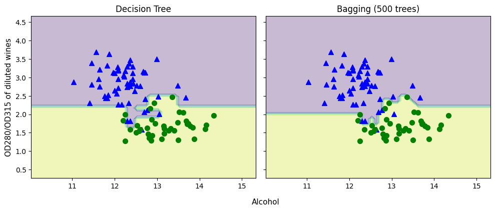

Notice: Bagging produces smoother decision boundaries.

4. Leveraging Weak Learners via Adaptive Boosting¶

Key Difference from Bagging¶

Aspect	Bagging	Boosting
Training	Parallel (independent trees)	Sequential (each tree corrects previous)
Focus	Reduce variance	Reduce bias
Base learners	Complex (deep trees)	Simple (stumps)
Data sensitivity	Robust to noise	Sensitive to outliers

How AdaBoost Works¶

Train a weak learner on weighted data (initially uniform weights)
Increase weights of misclassified samples
Train next learner on reweighted data
Combine all learners with weighted vote

Let’s walk through the weight update mechanism step by step:

# AdaBoost weight update walkthrough
print("AdaBoost Weight Update Mechanism")
print("=" * 50)

# Example: 10 samples with predictions
y = np.array([1, 1, 1, -1, -1, -1, 1, 1, 1, -1])     # True labels
yhat = np.array([1, 1, 1, -1, -1, -1, -1, -1, -1, -1])  # Predictions (3 errors)
correct = (y == yhat)
weights = np.full(10, 0.1)  # Initial uniform weights

print(f"True labels:    {y}")
print(f"Predictions:    {yhat}")
print(f"Correct?:       {correct.astype(int)}")
print(f"Initial weights: {weights}")

AdaBoost Weight Update Mechanism
==================================================
True labels:    [ 1  1  1 -1 -1 -1  1  1  1 -1]
Predictions:    [ 1  1  1 -1 -1 -1 -1 -1 -1 -1]
Correct?:       [1 1 1 1 1 1 0 0 0 1]
Initial weights: [0.1 0.1 0.1 0.1 0.1 0.1 0.1 0.1 0.1 0.1]

# Step 1: Calculate weighted error rate
epsilon = np.mean(~correct)  # Fraction of misclassified samples
print(f"\nStep 1: Weighted error rate")
print(f"  epsilon = {epsilon:.1f} (30% of samples misclassified)")


Step 1: Weighted error rate
  epsilon = 0.3 (30% of samples misclassified)

# Step 2: Calculate classifier weight
# Formula: alpha_j = 0.5 * ln((1 - epsilon) / epsilon)
alpha_j = 0.5 * np.log((1 - epsilon) / epsilon)
print(f"\nStep 2: Classifier weight")
print(f"  alpha_j = 0.5 * ln((1 - {epsilon}) / {epsilon})")
print(f"  alpha_j = {alpha_j:.3f}")
print(f"\n  Interpretation: Better classifiers get higher weights")


Step 2: Classifier weight
  alpha_j = 0.5 * ln((1 - 0.3) / 0.3)
  alpha_j = 0.424

  Interpretation: Better classifiers get higher weights

# Step 3: Update sample weights
# Correctly classified: w_i * exp(-alpha_j)
# Incorrectly classified: w_i * exp(+alpha_j)
update_if_correct = 0.1 * np.exp(-alpha_j * 1 * 1)
update_if_wrong = 0.1 * np.exp(-alpha_j * 1 * -1)

print(f"\nStep 3: Update sample weights")
print(f"  Weight if correct:   0.1 * exp(-{alpha_j:.3f}) = {update_if_correct:.4f}")
print(f"  Weight if incorrect: 0.1 * exp(+{alpha_j:.3f}) = {update_if_wrong:.4f}")

# Apply updates
weights = np.where(correct, update_if_correct, update_if_wrong)
print(f"\n  Updated weights (before normalization):")
print(f"  {np.round(weights, 4)}")

# Normalize
normalized_weights = weights / np.sum(weights)
print(f"\n  Normalized weights (sum to 1):")
print(f"  {np.round(normalized_weights, 4)}")
print(f"\n  Effect: Misclassified samples now have HIGHER weights!")


Step 3: Update sample weights
  Weight if correct:   0.1 * exp(-0.424) = 0.0655
  Weight if incorrect: 0.1 * exp(+0.424) = 0.1528

  Updated weights (before normalization):
  [0.0655 0.0655 0.0655 0.0655 0.0655 0.0655 0.1528 0.1528 0.1528 0.0655]

  Normalized weights (sum to 1):
  [0.0714 0.0714 0.0714 0.0714 0.0714 0.0714 0.1667 0.1667 0.1667 0.0714]

  Effect: Misclassified samples now have HIGHER weights!

Applying AdaBoost with scikit-learn¶

# AdaBoost uses shallow trees (stumps) as weak learners
tree = DecisionTreeClassifier(criterion='entropy', max_depth=1, random_state=1)

ada = AdaBoostClassifier(estimator=tree,
                         n_estimators=500,
                         learning_rate=0.1,
                         random_state=1)

# Train and evaluate single stump
tree = tree.fit(X_train, y_train)
y_train_pred = tree.predict(X_train)
y_test_pred = tree.predict(X_test)
tree_train = accuracy_score(y_train, y_train_pred)
tree_test = accuracy_score(y_test, y_test_pred)

# Train and evaluate AdaBoost
ada = ada.fit(X_train, y_train)
y_train_pred = ada.predict(X_train)
y_test_pred = ada.predict(X_test)
ada_train = accuracy_score(y_train, y_train_pred)
ada_test = accuracy_score(y_test, y_test_pred)

print("Results: Decision Stump vs AdaBoost")
print("=" * 50)
print(f"{'Model':<25} {'Train Acc':>12} {'Test Acc':>12}")
print("-" * 50)
print(f"{'Decision Stump':<25} {tree_train:>12.3f} {tree_test:>12.3f}")
print(f"{'AdaBoost (500 stumps)':<25} {ada_train:>12.3f} {ada_test:>12.3f}")
print("\n** Many weak learners combine into a strong learner! **")

Results: Decision Stump vs AdaBoost
==================================================
Model                        Train Acc     Test Acc
--------------------------------------------------
Decision Stump                   0.916        0.875
AdaBoost (500 stumps)            0.968        0.917

** Many weak learners combine into a strong learner! **

# Visualize decision boundaries: Stump vs AdaBoost
x_min, x_max = X_train[:, 0].min() - 1, X_train[:, 0].max() + 1
y_min, y_max = X_train[:, 1].min() - 1, X_train[:, 1].max() + 1
xx, yy = np.meshgrid(np.arange(x_min, x_max, 0.1),
                     np.arange(y_min, y_max, 0.1))

f, axarr = plt.subplots(1, 2, sharex='col', sharey='row', figsize=(10, 4))

for idx, clf, tt in zip([0, 1], [tree, ada], ['Decision Stump', 'AdaBoost (500 stumps)']):
    clf.fit(X_train, y_train)
    Z = clf.predict(np.c_[xx.ravel(), yy.ravel()])
    Z = Z.reshape(xx.shape)

    axarr[idx].contourf(xx, yy, Z, alpha=0.3)
    axarr[idx].scatter(X_train[y_train == 0, 0], X_train[y_train == 0, 1],
                       c='blue', marker='^', s=50)
    axarr[idx].scatter(X_train[y_train == 1, 0], X_train[y_train == 1, 1],
                       c='green', marker='o', s=50)
    axarr[idx].set_title(tt, fontsize=12)

axarr[0].set_ylabel('OD280/OD315 of diluted wines', fontsize=11)
plt.tight_layout()
plt.text(0, -0.15, s='Alcohol', ha='center', va='center', fontsize=11, transform=axarr[1].transAxes)
plt.show()

print("Notice: AdaBoost creates complex boundaries from simple stumps.")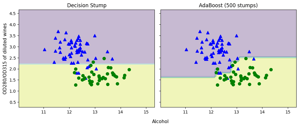

Notice: AdaBoost creates complex boundaries from simple stumps.

5. Gradient Boosting and XGBoost¶

Gradient Boosting¶

Similar to AdaBoost but:

Fits new models to residual errors (gradients of the loss function)
Uses gradient descent to minimize a loss function
More flexible loss functions possible

XGBoost: Extreme Gradient Boosting¶

XGBoost is an optimized implementation of gradient boosting that provides:

Speed: Parallel processing and cache optimization
Regularization: L1 and L2 regularization to prevent overfitting
Missing values: Automatic handling of missing data
Tree pruning: Uses max_depth and prunes trees backward

try:
    import xgboost as xgb
    
    model = xgb.XGBClassifier(
        n_estimators=1000,
        learning_rate=0.01,
        max_depth=4,
        random_state=1,
        use_label_encoder=False,
        eval_metric='logloss'
    )
    
    gbm = model.fit(X_train, y_train)
    
    y_train_pred = gbm.predict(X_train)
    y_test_pred = gbm.predict(X_test)
    
    gbm_train = accuracy_score(y_train, y_train_pred)
    gbm_test = accuracy_score(y_test, y_test_pred)
    
    print(f"XGBoost train/test accuracies: {gbm_train:.3f}/{gbm_test:.3f}")
    
except ImportError:
    print("XGBoost not installed. Install with: pip install xgboost")
    gbm_train, gbm_test = None, None

XGBoost train/test accuracies: 0.968/0.917

Comparison: Bagging vs Boosting¶

Aspect	Bagging	Boosting
Training	Parallel	Sequential
Focus	Reduce variance	Reduce bias
Base learners	Complex (deep trees)	Simple (stumps)
Overfitting	Resistant	Can overfit
Data sensitivity	Robust to noise	Sensitive to outliers

When to Use Each Method¶

Bagging / Random Forests:

High variance models
Noisy data
Need interpretability

AdaBoost / Gradient Boosting:

High bias models
Clean data
Maximum predictive performance

6. Summary¶

Key Takeaways¶

Ensembles work by combining classifiers with diverse, uncorrelated errors
Majority voting combines different algorithms through votes or probabilities
Bagging reduces variance by training on bootstrap samples (parallel)
AdaBoost sequentially focuses on misclassified examples (sequential)
Gradient boosting minimizes loss by fitting to residuals
XGBoost provides optimized gradient boosting with regularization

Comparison of Methods¶

Method	Approach	Best For
Voting	Different algorithms	Combining diverse models
Bagging	Bootstrap samples	Reducing variance
AdaBoost	Reweight samples	Sequential correction
XGBoost	Gradient descent	Maximum performance

References¶

Primary Source¶

Raschka, S., Liu, Y., & Mirjalili, V. (2022). Machine Learning with PyTorch and Scikit-Learn. Packt Publishing. Chapter 7.
Code: https://github.com/rasbt/machine-learning-book/tree/main/ch07

Academic Papers¶

Breiman, L. (1996). Bagging Predictors. Machine Learning, 24(2), 123-140.
Freund, Y. & Schapire, R. (1997). A Decision-Theoretic Generalization of On-Line Learning. Journal of Computer and System Sciences.
Chen, T. & Guestrin, C. (2016). XGBoost: A Scalable Tree Boosting System. KDD.