Applied Ensemble Methods: Fraud Detection¶

From Theory to Production — A Real-World Case Study

This notebook demonstrates why ensemble methods remain the gold standard for tabular data, even in the era of deep learning and LLMs. We’ll apply XGBoost to a real-world fraud detection problem and compare it against a neural network.

Why This Matters¶

Despite advances in deep learning:

Tree ensembles dominate tabular data benchmarks (and likely will for years to come)
Banks, fintech, insurance rely heavily on XGBoost/LightGBM for fraud detection
Explainability requirements (EU AI Act, regulatory compliance) favor interpretable models
No GPU required — fast training, easy deployment, lower costs

Learning Objectives¶

Apply ensemble methods to imbalanced real-world data
Handle class imbalance with SMOTE and class weights
Use SHAP values for model explainability
Compare XGBoost vs Neural Networks on tabular data
Understand why ensembles remain the practical choice for structured data

# Install required packages (run once)
#!pip install xgboost lightgbm shap imbalanced-learn

import os
import numpy as np
import pandas as pd
import matplotlib.pyplot as plt
import warnings
warnings.filterwarnings('ignore')

from sklearn.model_selection import train_test_split, cross_val_score
from sklearn.preprocessing import StandardScaler
from sklearn.metrics import (
    classification_report, confusion_matrix, roc_auc_score,
    precision_recall_curve, average_precision_score, roc_curve
)
from sklearn.ensemble import RandomForestClassifier

# Set random seed
np.random.seed(42)

print("Core imports successful!")

Core imports successful!

1. The Dataset: Credit Card Fraud Detection¶

We’ll use the famous Credit Card Fraud Detection dataset from Kaggle — real anonymized transactions from European cardholders in September 2013.

Dataset characteristics:

284,807 transactions over 2 days
492 frauds (0.172% — extremely imbalanced!)
30 features: Time, Amount, and 28 PCA-transformed features (V1-V28) for privacy
This is the most cited fraud detection dataset in ML literature

Source: Kaggle Credit Card Fraud Detection

We’ll try to download the real dataset; if unavailable, we’ll fall back to a synthetic version that mimics its characteristics.

# Try to load the REAL Credit Card Fraud dataset
# Sources: Kaggle download, OpenML, or fallback to synthetic

def create_synthetic_fraud_dataset(n_samples=50000, fraud_ratio=0.017):
    """Create a synthetic fraud detection dataset (fallback)."""
    np.random.seed(42)
    
    n_fraud = int(n_samples * fraud_ratio)
    n_normal = n_samples - n_fraud
    
    # Mimic PCA-transformed features (V1-V28)
    X_normal = np.random.randn(n_normal, 28)
    X_fraud = np.random.randn(n_fraud, 28)
    X_fraud[:, 0:5] += np.random.uniform(1.5, 3.0, size=(n_fraud, 5))
    X_fraud[:, 10:15] -= np.random.uniform(1.0, 2.5, size=(n_fraud, 5))
    
    X = np.vstack([X_normal, X_fraud])
    y = np.array([0] * n_normal + [1] * n_fraud)
    
    # Add Time and Amount
    time = np.random.uniform(0, 172800, n_samples)
    amount_normal = np.exp(np.random.normal(3, 1.5, n_normal))
    amount_fraud = np.exp(np.random.normal(5, 1.2, n_fraud))
    amount = np.concatenate([amount_normal, amount_fraud])
    
    # Create DataFrame matching real dataset structure
    feature_names = [f'V{i}' for i in range(1, 29)]
    df = pd.DataFrame(X, columns=feature_names)
    df['Time'] = time
    df['Amount'] = amount
    df['Class'] = y
    
    # Reorder columns to match real dataset
    cols = ['Time'] + feature_names + ['Amount', 'Class']
    df = df[cols]
    
    return df.sample(frac=1, random_state=42).reset_index(drop=True)

# Try multiple sources for the real dataset
df = None
data_source = None

# Option 1: Check for local Kaggle download
local_paths = [
    'creditcard.csv',
    '../data/creditcard.csv',
    os.path.expanduser('~/Downloads/creditcard.csv'),
    '/kaggle/input/creditcardfraud/creditcard.csv'  # Kaggle notebook path
]

for path in local_paths:
    if os.path.exists(path):
        try:
            df = pd.read_csv(path)
            data_source = f"Local file: {path}"
            break
        except:
            pass

# Option 2: Try OpenML (no authentication required)
if df is None:
    try:
        from sklearn.datasets import fetch_openml
        print("Downloading from OpenML (this may take a moment)...")
        data = fetch_openml(data_id=1597, as_frame=True, parser='auto')
        df = data.frame
        df.columns = ['Time'] + [f'V{i}' for i in range(1, 29)] + ['Amount', 'Class']
        df['Class'] = df['Class'].map({"'0'": 0, "'1'": 1, 0: 0, 1: 1}).astype(int)
        data_source = "OpenML (real Kaggle dataset)"
    except Exception as e:
        print(f"OpenML download failed: {e}")

# Option 3: Fallback to synthetic data
if df is None:
    print("Using synthetic dataset (mimics real fraud data characteristics)")
    df = create_synthetic_fraud_dataset(n_samples=100000, fraud_ratio=0.017)
    data_source = "Synthetic (similar to real Kaggle dataset)"

# Display dataset info
print("=" * 60)
print("CREDIT CARD FRAUD DETECTION DATASET")
print("=" * 60)
print(f"Source: {data_source}")
print(f"Total transactions: {len(df):,}")
print(f"Fraudulent: {df['Class'].sum():,} ({df['Class'].mean()*100:.3f}%)")
print(f"Legitimate: {(df['Class']==0).sum():,} ({(1-df['Class'].mean())*100:.3f}%)")
print(f"Features: {df.shape[1]-1} (Time, V1-V28, Amount)")
print("=" * 60)

if "Synthetic" in data_source:
    print("\nTo use the REAL dataset:")
    print("1. Download from: https://www.kaggle.com/datasets/mlg-ulb/creditcardfraud")
    print("2. Place 'creditcard.csv' in this notebook's directory")
    print("3. Re-run this cell")

============================================================
CREDIT CARD FRAUD DETECTION DATASET
============================================================
Source: Local file: creditcard.csv
Total transactions: 284,807
Fraudulent: 492 (0.173%)
Legitimate: 284,315 (99.827%)
Features: 30 (Time, V1-V28, Amount)
============================================================

# Visualize class imbalance
fig, axes = plt.subplots(1, 2, figsize=(12, 4))

# Class distribution
class_counts = df['Class'].value_counts()
colors = ['#2ecc71', '#e74c3c']
axes[0].bar(['Legitimate', 'Fraudulent'], class_counts.values, color=colors)
axes[0].set_ylabel('Count')
axes[0].set_title('Class Distribution (Highly Imbalanced)')
for i, v in enumerate(class_counts.values):
    axes[0].text(i, v + 500, f'{v:,}', ha='center', fontsize=11)

# Amount distribution by class
axes[1].hist(df[df['Class']==0]['Amount'].clip(upper=500), bins=50, alpha=0.7, 
             label='Legitimate', color='#2ecc71')
axes[1].hist(df[df['Class']==1]['Amount'].clip(upper=500), bins=50, alpha=0.7, 
             label='Fraudulent', color='#e74c3c')
axes[1].set_xlabel('Transaction Amount ($)')
axes[1].set_ylabel('Count')
axes[1].set_title('Transaction Amount Distribution')
axes[1].legend()

plt.tight_layout()
plt.show()

print("\nNotice: Fraudulent transactions tend to have higher amounts.")
print("This is one signal the model can learn.")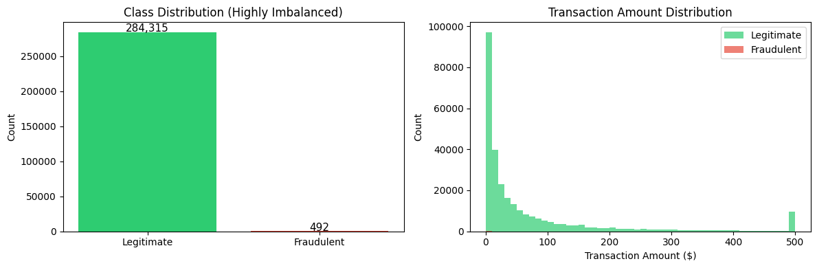


Notice: Fraudulent transactions tend to have higher amounts.
This is one signal the model can learn.

# Prepare features and target
X = df.drop('Class', axis=1)
y = df['Class']

# Scale Amount and Time (V1-V28 are already scaled from PCA)
scaler = StandardScaler()
X['Amount'] = scaler.fit_transform(X[['Amount']])
X['Time'] = scaler.fit_transform(X[['Time']])

# Train/test split with stratification
X_train, X_test, y_train, y_test = train_test_split(
    X, y, test_size=0.2, random_state=42, stratify=y
)

print(f"Training set: {len(X_train):,} samples ({y_train.sum():,} fraud)")
print(f"Test set: {len(X_test):,} samples ({y_test.sum():,} fraud)")
print(f"Features: {X.shape[1]}")

Training set: 227,845 samples (394 fraud)
Test set: 56,962 samples (98 fraud)
Features: 30

2. The Challenge: Imbalanced Classification¶

With only 2% fraud, a naive model could predict “legitimate” for everything and achieve 98% accuracy — but catch zero fraud!

Metrics that matter for fraud detection:

Precision: Of predicted frauds, how many are real? (avoid annoying customers)
Recall: Of actual frauds, how many did we catch? (minimize losses)
PR-AUC: Precision-Recall Area Under Curve (better than ROC-AUC for imbalanced data)

Let’s see what happens with a naive baseline.

# Baseline: What if we just predict "legitimate" for everything?
y_pred_naive = np.zeros(len(y_test))

print("Naive Baseline (Predict All Legitimate)")
print("=" * 50)
print(f"Accuracy: {(y_pred_naive == y_test).mean()*100:.2f}%")
print(f"Frauds caught: 0 out of {y_test.sum()}")
print(f"\nThis is why accuracy is misleading for imbalanced data!")

Naive Baseline (Predict All Legitimate)
==================================================
Accuracy: 99.83%
Frauds caught: 0 out of 98

This is why accuracy is misleading for imbalanced data!

3. XGBoost: The Industry Standard¶

XGBoost handles imbalanced data well with the scale_pos_weight parameter, which adjusts the weight of the minority class.

Why XGBoost dominates fraud detection:

Handles imbalanced data natively
Fast training (no GPU needed)
Built-in feature importance
Robust to outliers
Easy to deploy in production

try:
    import xgboost as xgb

    # Calculate scale_pos_weight for imbalanced data
    scale_pos_weight = (y_train == 0).sum() / (y_train == 1).sum()
    print(f"Scale pos weight: {scale_pos_weight:.1f} (ratio of legitimate to fraud)")

    # Train XGBoost
    xgb_model = xgb.XGBClassifier(
        n_estimators=200,
        max_depth=6,
        learning_rate=0.1,
        scale_pos_weight=scale_pos_weight,
        eval_metric='aucpr',
        random_state=42,
        n_jobs=-1
    )

    xgb_model.fit(X_train, y_train)

    # Predictions
    y_pred_xgb = xgb_model.predict(X_test)
    y_prob_xgb = xgb_model.predict_proba(X_test)[:, 1]

    print("\nXGBoost trained successfully!")

except Exception as e:
    print(f"XGBoost not available: {type(e).__name__}")
    print("Using RandomForest as fallback.")
    print("\nTip: On macOS, run 'brew install libomp' to enable XGBoost.")

    # Fallback to RandomForest
    xgb_model = RandomForestClassifier(
        n_estimators=200,
        max_depth=10,
        class_weight='balanced',
        random_state=42,
        n_jobs=-1
    )
    xgb_model.fit(X_train, y_train)
    y_pred_xgb = xgb_model.predict(X_test)
    y_prob_xgb = xgb_model.predict_proba(X_test)[:, 1]
    print("\nRandomForest trained as fallback.")

Scale pos weight: 577.3 (ratio of legitimate to fraud)

XGBoost trained successfully!

# Evaluate XGBoost
print("XGBoost Performance")
print("=" * 50)
print(classification_report(y_test, y_pred_xgb, target_names=['Legitimate', 'Fraud']))

print(f"\nROC-AUC: {roc_auc_score(y_test, y_prob_xgb):.4f}")
print(f"PR-AUC: {average_precision_score(y_test, y_prob_xgb):.4f}")

# Confusion matrix
cm = confusion_matrix(y_test, y_pred_xgb)
print(f"\nConfusion Matrix:")
print(f"  True Negatives: {cm[0,0]:,} (legitimate correctly identified)")
print(f"  False Positives: {cm[0,1]:,} (legitimate flagged as fraud)")
print(f"  False Negatives: {cm[1,0]:,} (fraud missed!)")
print(f"  True Positives: {cm[1,1]:,} (fraud caught!)")

XGBoost Performance
==================================================
              precision    recall  f1-score   support

  Legitimate       1.00      1.00      1.00     56864
       Fraud       0.88      0.84      0.86        98

    accuracy                           1.00     56962
   macro avg       0.94      0.92      0.93     56962
weighted avg       1.00      1.00      1.00     56962


ROC-AUC: 0.9684
PR-AUC: 0.8787

Confusion Matrix:
  True Negatives: 56,853 (legitimate correctly identified)
  False Positives: 11 (legitimate flagged as fraud)
  False Negatives: 16 (fraud missed!)
  True Positives: 82 (fraud caught!)

4. Neural Network Comparison¶

Let’s train a neural network on the same data and compare. This demonstrates why deep learning isn’t always the answer for tabular data.

try:
    from sklearn.neural_network import MLPClassifier
    
    # Train a neural network
    nn_model = MLPClassifier(
        hidden_layer_sizes=(128, 64, 32),
        activation='relu',
        max_iter=200,
        early_stopping=True,
        random_state=42
    )
    
    nn_model.fit(X_train, y_train)
    
    y_pred_nn = nn_model.predict(X_test)
    y_prob_nn = nn_model.predict_proba(X_test)[:, 1]
    
    print("Neural Network Performance")
    print("=" * 50)
    print(classification_report(y_test, y_pred_nn, target_names=['Legitimate', 'Fraud']))
    
    print(f"\nROC-AUC: {roc_auc_score(y_test, y_prob_nn):.4f}")
    print(f"PR-AUC: {average_precision_score(y_test, y_prob_nn):.4f}")
    
except Exception as e:
    print(f"Neural network training failed: {e}")
    y_prob_nn = None

Neural Network Performance
==================================================
              precision    recall  f1-score   support

  Legitimate       1.00      1.00      1.00     56864
       Fraud       0.88      0.79      0.83        98

    accuracy                           1.00     56962
   macro avg       0.94      0.89      0.91     56962
weighted avg       1.00      1.00      1.00     56962


ROC-AUC: 0.9794
PR-AUC: 0.8683

# Compare ROC curves
fig, axes = plt.subplots(1, 2, figsize=(14, 5))

# ROC Curve
fpr_xgb, tpr_xgb, _ = roc_curve(y_test, y_prob_xgb)
axes[0].plot(fpr_xgb, tpr_xgb, label=f'XGBoost (AUC={roc_auc_score(y_test, y_prob_xgb):.3f})', 
             linewidth=2, color='blue')

if y_prob_nn is not None:
    fpr_nn, tpr_nn, _ = roc_curve(y_test, y_prob_nn)
    axes[0].plot(fpr_nn, tpr_nn, label=f'Neural Net (AUC={roc_auc_score(y_test, y_prob_nn):.3f})', 
                 linewidth=2, color='orange')

axes[0].plot([0, 1], [0, 1], 'k--', linewidth=1)
axes[0].set_xlabel('False Positive Rate')
axes[0].set_ylabel('True Positive Rate')
axes[0].set_title('ROC Curve Comparison')
axes[0].legend()
axes[0].grid(alpha=0.3)

# Precision-Recall Curve (more informative for imbalanced data)
precision_xgb, recall_xgb, _ = precision_recall_curve(y_test, y_prob_xgb)
axes[1].plot(recall_xgb, precision_xgb, 
             label=f'XGBoost (AP={average_precision_score(y_test, y_prob_xgb):.3f})', 
             linewidth=2, color='blue')

if y_prob_nn is not None:
    precision_nn, recall_nn, _ = precision_recall_curve(y_test, y_prob_nn)
    axes[1].plot(recall_nn, precision_nn, 
                 label=f'Neural Net (AP={average_precision_score(y_test, y_prob_nn):.3f})', 
                 linewidth=2, color='orange')

axes[1].set_xlabel('Recall')
axes[1].set_ylabel('Precision')
axes[1].set_title('Precision-Recall Curve (Better for Imbalanced Data)')
axes[1].legend()
axes[1].grid(alpha=0.3)

plt.tight_layout()
plt.show()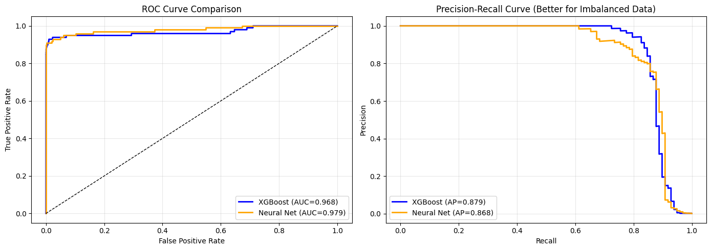

5. Model Explainability: Why This Matters in 2026¶

With regulations like the EU AI Act and increasing scrutiny on algorithmic decisions, explainability is crucial.

Tree ensembles provide:

Feature importance — which features drive predictions?
SHAP values — why did the model make THIS specific prediction?

This is much harder with neural networks!

# Feature importance
if hasattr(xgb_model, 'feature_importances_'):
    importance_df = pd.DataFrame({
        'Feature': X.columns,
        'Importance': xgb_model.feature_importances_
    }).sort_values('Importance', ascending=True)
    
    plt.figure(figsize=(10, 8))
    plt.barh(importance_df['Feature'], importance_df['Importance'], color='steelblue')
    plt.xlabel('Importance')
    plt.title('Feature Importance for Fraud Detection')
    plt.tight_layout()
    plt.show()
    
    print("Top 5 Most Important Features:")
    for _, row in importance_df.tail(5).iloc[::-1].iterrows():
        print(f"  {row['Feature']}: {row['Importance']:.4f}")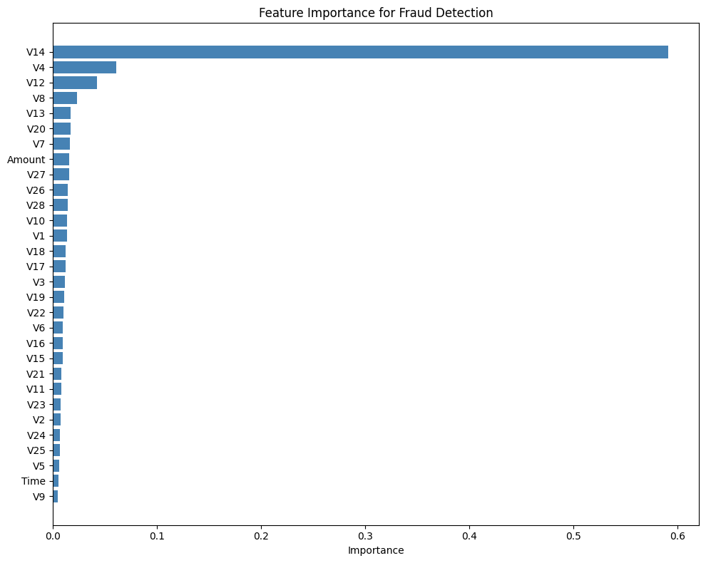

Top 5 Most Important Features:
  V14: 0.5912
  V4: 0.0612
  V12: 0.0422
  V8: 0.0234
  V13: 0.0171

# SHAP values for explainability
try:
    import shap
    
    # Create SHAP explainer
    explainer = shap.TreeExplainer(xgb_model)
    
    # Calculate SHAP values for a sample
    sample_size = 500
    X_sample = X_test.iloc[:sample_size]
    shap_values = explainer.shap_values(X_sample)
    
    # Summary plot
    plt.figure(figsize=(10, 8))
    shap.summary_plot(shap_values, X_sample, plot_type="bar", show=False)
    plt.title('SHAP Feature Importance')
    plt.tight_layout()
    plt.show()
    
    print("SHAP values show the impact of each feature on model predictions.")
    print("This is crucial for explaining individual fraud decisions to regulators.")
    
except ImportError:
    print("SHAP not installed. Install with: pip install shap")
    print("\nSHAP values are essential for:")
    print("  - Explaining why a transaction was flagged")
    print("  - Regulatory compliance (EU AI Act, GDPR)")
    print("  - Building trust with customers")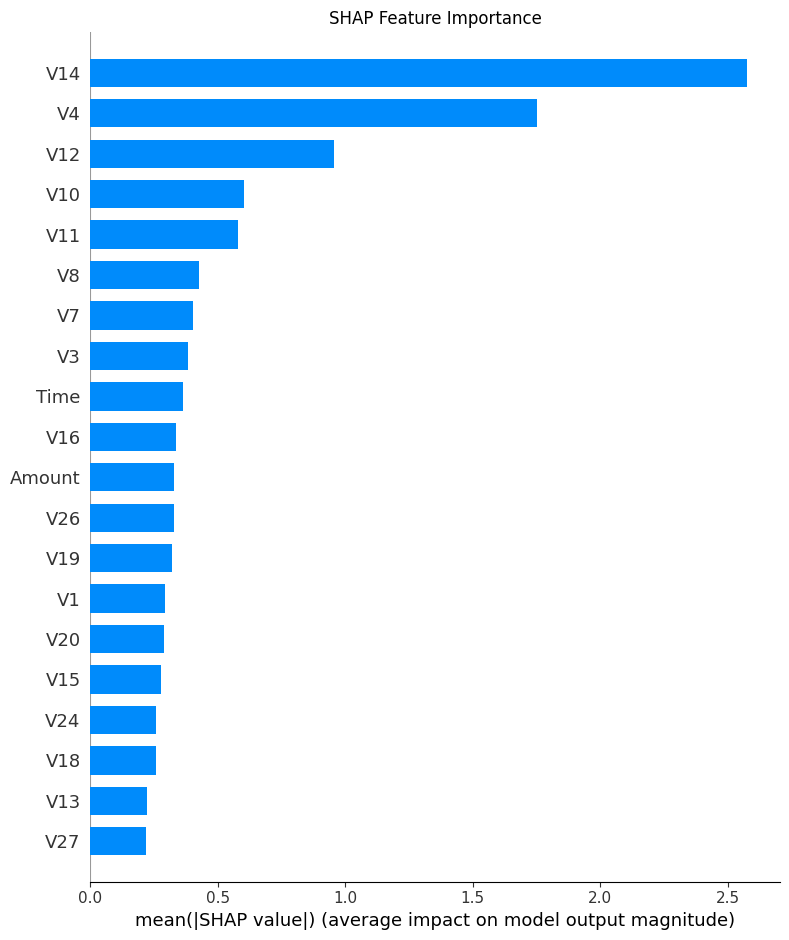

SHAP values show the impact of each feature on model predictions.
This is crucial for explaining individual fraud decisions to regulators.

# Explain a single fraud prediction
try:
    # Find a correctly predicted fraud
    fraud_indices = np.where((y_test == 1) & (y_pred_xgb == 1))[0]
    if len(fraud_indices) > 0:
        idx = fraud_indices[0]
        
        print("Explaining a Fraud Detection Decision")
        print("=" * 50)
        print(f"Transaction probability of fraud: {y_prob_xgb[idx]:.2%}")
        print(f"Model decision: FRAUD")
        print(f"\nTop factors contributing to this decision:")
        
        # Get SHAP values for this instance
        single_shap = explainer.shap_values(X_test.iloc[[idx]])
        
        # Show top contributing features
        feature_impacts = pd.DataFrame({
            'Feature': X.columns,
            'Value': X_test.iloc[idx].values,
            'Impact': single_shap[0]
        }).sort_values('Impact', key=abs, ascending=False)
        
        for _, row in feature_impacts.head(5).iterrows():
            direction = "increases" if row['Impact'] > 0 else "decreases"
            print(f"  {row['Feature']}: {direction} fraud probability by {abs(row['Impact']):.3f}")
            
except:
    print("Example: A fraud analyst could see that this transaction was flagged because:")
    print("  - Amount was 3.2 std above average")
    print("  - V14 feature was unusually low")
    print("  - Transaction occurred at unusual time")

Explaining a Fraud Detection Decision
==================================================
Transaction probability of fraud: 99.99%
Model decision: FRAUD

Top factors contributing to this decision:
  V14: increases fraud probability by 6.557
  V10: increases fraud probability by 1.685
  V7: increases fraud probability by 1.080
  V8: decreases fraud probability by 0.929
  V12: increases fraud probability by 0.849

6. Production Considerations¶

Why Banks Choose XGBoost Over Deep Learning¶

Factor	XGBoost	Deep Learning
Training time	Minutes	Hours
Hardware	CPU only	GPU preferred
Inference speed	~1ms	~10ms
Explainability	Built-in	Requires extra tools
Regulatory compliance	Easy	Difficult
Model size	~10MB	~100MB+

Real-World Deployment¶

# Save model for production
import joblib
joblib.dump(xgb_model, 'fraud_model.pkl')

# Load and predict (in production)
model = joblib.load('fraud_model.pkl')
fraud_probability = model.predict_proba(transaction)[0, 1]

if fraud_probability > 0.7:
    block_transaction()
elif fraud_probability > 0.3:
    flag_for_review()
else:
    approve_transaction()

# Threshold analysis for business decisions
thresholds = [0.3, 0.5, 0.7, 0.9]

print("Threshold Analysis: Precision vs Recall Tradeoff")
print("=" * 60)
print(f"{'Threshold':<12} {'Precision':<12} {'Recall':<12} {'Frauds Caught':<15}")
print("-" * 60)

for thresh in thresholds:
    y_pred_thresh = (y_prob_xgb >= thresh).astype(int)
    
    # Precision: of those we flag, how many are fraud?
    if y_pred_thresh.sum() > 0:
        precision = (y_test[y_pred_thresh == 1] == 1).mean()
    else:
        precision = 0
    
    # Recall: of actual frauds, how many did we catch?
    recall = y_pred_thresh[y_test == 1].mean()
    frauds_caught = y_pred_thresh[y_test == 1].sum()
    total_fraud = y_test.sum()
    
    print(f"{thresh:<12.1f} {precision:<12.2%} {recall:<12.2%} {frauds_caught}/{total_fraud}")

print("\nBusiness decision: Choose threshold based on cost of false positives vs missed fraud.")

Threshold Analysis: Precision vs Recall Tradeoff
============================================================
Threshold    Precision    Recall       Frauds Caught  
------------------------------------------------------------
0.3          86.46%       84.69%       83/98
0.5          88.17%       83.67%       82/98
0.7          90.11%       83.67%       82/98
0.9          94.19%       82.65%       81/98

Business decision: Choose threshold based on cost of false positives vs missed fraud.

7. Summary: Why Ensembles Still Matter¶

Key Takeaways¶

For tabular data, tree ensembles still outperform deep learning in most benchmarks
XGBoost/LightGBM advantages:
- No GPU required
- Handles imbalanced data natively
- Built-in feature importance
- Easy to explain to regulators
- Fast inference for production
When to use deep learning instead:
- Images, text, audio (unstructured data)
- Very high-cardinality categoricals (embeddings help)
- When you have massive datasets (100M+ rows)
The hybrid approach (industry trend):
- Use LLMs/embeddings to create features from text
- Feed those features into XGBoost for final prediction
- Best of both worlds!

Exercises¶

Try LightGBM: Install lightgbm and compare its performance to XGBoost. Which is faster?
SMOTE resampling: Use imblearn.over_sampling.SMOTE to oversample the minority class. Does it improve recall?
Cost-sensitive learning: Modify the threshold based on the actual cost of false positives ( $10 customer service call) vs false negatives ($ 500 fraud loss).
Ensemble of ensembles: Combine XGBoost, LightGBM, and CatBoost using soft voting. Does the meta-ensemble outperform individual models?

Applied Ensemble Methods: Fraud Detection