Chapter 19 - Reinforcement Learning for Decision Making in Complex Environments
from IPython.display import Image
%matplotlib inline
Implementing our first RL algorithm
Working with the existing environments in OpenAI Gym
Purpose of This Section
Demonstrates how to implement Q-learning to solve a grid-world task.
Uses OpenAI Gym environments to provide a practical RL simulation framework.
Focuses on tabular Q-learning, the most basic model-free RL method.
Introducing OpenAI Gym Toolkit
OpenAI Gym: A library of environments for benchmarking RL algorithms.
Includes environments from simple to complex (e.g.,
CartPole,MountainCar, robotics).Gym provides:
A unified API for agent-environment interaction.
Tools for rendering and stepping through environments.
# !pip install gymLooking in indexes: https://pypi.org/simple, https://pypi.ngc.nvidia.com
Collecting gym
Downloading gym-0.26.2.tar.gz (721 kB)
━━━━━━━━━━━━━━━━━━━━━━━━━━━━━━━━━━━━━━ 721.7/721.7 kB 22.6 MB/s eta 0:00:00
Installing build dependencies ... done
Getting requirements to build wheel ... done
Preparing metadata (pyproject.toml) ... done
Requirement already satisfied: numpy>=1.18.0 in /usr/local/lib/python3.10/dist-packages (from gym) (1.22.2)
Requirement already satisfied: cloudpickle>=1.2.0 in /usr/local/lib/python3.10/dist-packages (from gym) (2.2.1)
Collecting gym_notices>=0.0.4 (from gym)
Downloading gym_notices-0.0.8-py3-none-any.whl.metadata (1.0 kB)
Downloading gym_notices-0.0.8-py3-none-any.whl (3.0 kB)
Building wheels for collected packages: gym
Building wheel for gym (pyproject.toml) ... done
Created wheel for gym: filename=gym-0.26.2-py3-none-any.whl size=827745 sha256=4d987f726634dfbd8a8da8912681f3deb5a534e4e190767b465f9daa6e208361
Stored in directory: /tmp/pip-ephem-wheel-cache-nxita8rx/wheels/b9/22/6d/3e7b32d98451b4cd9d12417052affbeeeea012955d437da1da
Successfully built gym
Installing collected packages: gym_notices, gym
Successfully installed gym-0.26.2 gym_notices-0.0.8
WARNING: Running pip as the 'root' user can result in broken permissions and conflicting behaviour with the system package manager, possibly rendering your system unusable. It is recommended to use a virtual environment instead: https://pip.pypa.io/warnings/venv. Use the --root-user-action option if you know what you are doing and want to suppress this warning.
Working with Gym Environments
Use
gym.make(env_name)to load an environment.Common API methods:
env.reset()— initializes a new episode, returns initial observation.env.step(action)— executes an action, returns:next_state,reward,done,info
env.render()— (optional) visualizes the environment state.
Spaces:
env.observation_space— defines state format (e.g.,Box)env.action_space— defines possible actions (e.g.,Discrete)
The Environment: CartPole-v1
Classic RL task where a cart must balance a pole using left/right moves.
States (
Box(4,)): Continuous vector of 4 values (cart position, velocity, pole angle, and pole tip’s velocity) for min and max eachActions:
0(move left),1(move right)
Image(filename='figures/19_06.png', width=600)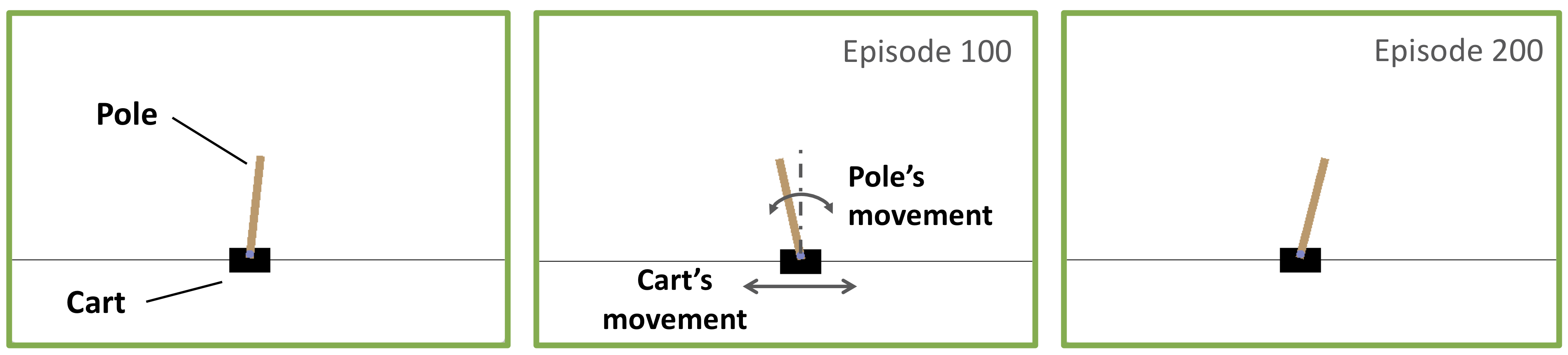
import gym

env = gym.make('CartPole-v1')
env.observation_space
Box([-4.8000002e+00 -3.4028235e+38 -4.1887903e-01 -3.4028235e+38], [4.8000002e+00 3.4028235e+38 4.1887903e-01 3.4028235e+38], (4,), float32)env.action_spaceDiscrete(2)# Set the pole’s starting state (S0)
env.reset()(array([-0.00863925, 0.02971761, -0.02400191, -0.04376195], dtype=float32),
{})Every time we call env.step(), it returns:
An array for the new state (or observations)
A reward (a scalar value of type
float)A termination flag (
TrueorFalse)A Python dictionary containing auxiliary information
# Push the cart to the left
env.step(action=0)
(array([-0.00804489, -0.16505209, -0.02487715, 0.24125256], dtype=float32),
1.0,
False,
False,
{})A grid world example
Image(filename='figures/19_07.png', width=600)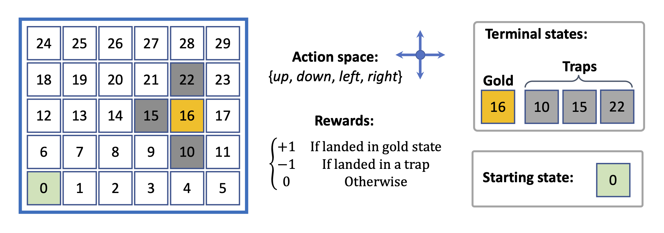
Image(filename='figures/19_08.png', width=600)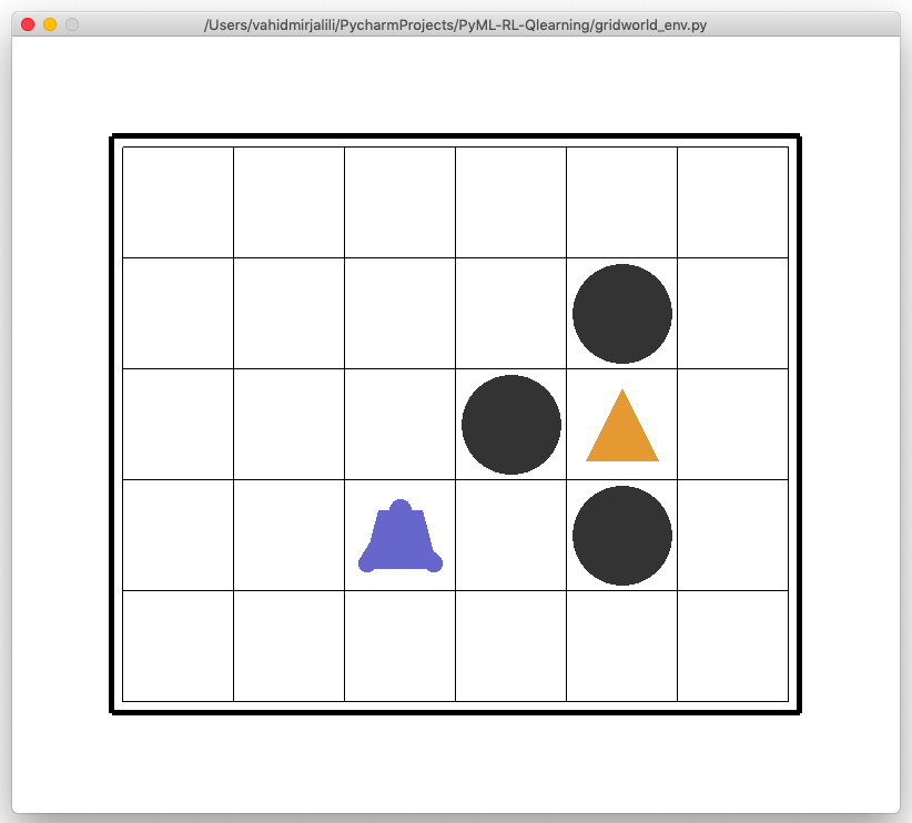
# gridworld_env.py
# Custom GridWorld environment - modernized for newer Gym
# Based on code from "Python Machine Learning, PyTorch Edition" (Raschka et al.)

import numpy as np
import gym
from gym import spaces
from collections import defaultdict
import time
import os
import pickle
# Visualization by matplotlib if built-in rendering is unavailable
import matplotlib.pyplot as plt
import matplotlib.patches as patches

try:
    from gym.envs.classic_control import rendering  # Classic gym
except ImportError:
    rendering = None  # Safe fallback for headless/Colab environments

CELL_SIZE = 100
MARGIN = 10


# Utility to get cell coordinates
def get_coords(row, col, loc='center'):
    xc = (col + 1.5) * CELL_SIZE
    yc = (row + 1.5) * CELL_SIZE

    if loc == 'center':
        return xc, yc
    elif loc == 'interior_corners':
        half = CELL_SIZE // 2 - MARGIN
        xl, xr = xc - half, xc + half
        yt, yb = yc - half, yc + half
        return [(xl, yt), (xr, yt), (xr, yb), (xl, yb)]
    elif loc == 'interior_triangle':
        return [
            (xc, yc + CELL_SIZE // 3),
            (xc + CELL_SIZE // 3, yc - CELL_SIZE // 3),
            (xc - CELL_SIZE // 3, yc - CELL_SIZE // 3),
        ]


# Utility to draw visual elements
def draw_object(coords_list):
    if rendering is None:
        return None

    if len(coords_list) == 1:  # circle
        obj = rendering.make_circle(int(0.45 * CELL_SIZE))
        transform = rendering.Transform()
        obj.add_attr(transform)
        transform.set_translation(*coords_list[0])
        obj.set_color(0.2, 0.2, 0.2)
    elif len(coords_list) == 3:  # triangle
        obj = rendering.FilledPolygon(coords_list)
        obj.set_color(0.9, 0.6, 0.2)
    else:  # polygon
        obj = rendering.FilledPolygon(coords_list)
        obj.set_color(0.4, 0.4, 0.8)

    return obj


class GridWorldEnv(gym.Env):
    """
    Custom GridWorld environment for simple reinforcement learning experiments.
    Grid contains:
    - Agent (starts at top-left)
    - Gold (goal, +1 reward)
    - Traps (fail states, -1 reward)
    """
    metadata = {"render_modes": ["human", "rgb_array"]}

    def __init__(self, num_rows=4, num_cols=6, delay=0.05):
        super().__init__()

        self.num_rows = num_rows
        self.num_cols = num_cols
        self.nS = num_rows * num_cols
        self.nA = 4  # up, right, down, left
        self.delay = delay

        self.action_space = spaces.Discrete(self.nA)
        self.observation_space = spaces.Discrete(self.nS)

        # Mapping between state index and grid positions
        self.grid2state = {(r, c): r * num_cols + c for r in range(num_rows) for c in range(num_cols)}
        self.state2grid = {v: k for k, v in self.grid2state.items()}

        # Goal and traps
        self.gold_cell = (num_rows // 2, num_cols - 2)
        self.trap_cells = [
            (self.gold_cell[0] + 1, self.gold_cell[1]),
            (self.gold_cell[0], self.gold_cell[1] - 1),
            (self.gold_cell[0] - 1, self.gold_cell[1])
        ]
        self.terminal_states = [self.grid2state[self.gold_cell]] + [self.grid2state[c] for c in self.trap_cells]

        # Initial state
        self.start_state = 0
        self.state = self.start_state

        # Transition model (deterministic)
        self.P = self._build_transition_model()

        # Viewer for rendering
        self.viewer = None
        if rendering is not None:
            self._build_display()

    # Build the transition probability
    def _build_transition_model(self):
        P = defaultdict(dict)

        for s in range(self.nS):
            row, col = self.state2grid[s]
            P[s] = defaultdict(list)

            for a in range(self.nA):
                new_row, new_col = row, col
                if a == 0: new_row = max(0, row - 1)       # up
                elif a == 1: new_col = min(self.num_cols - 1, col + 1)  # right
                elif a == 2: new_row = min(self.num_rows - 1, row + 1)  # down
                elif a == 3: new_col = max(0, col - 1)     # left

                next_state = self.grid2state[(new_row, new_col)]
                reward = 0.0
                done = False

                if next_state in self.terminal_states:
                    reward = 1.0 if next_state == self.grid2state[self.gold_cell] else -1.0
                    done = True

                if s in self.terminal_states:
                    # Terminal state is absorbing
                    P[s][a] = [(1.0, s, 0.0, True)]
                else:
                    P[s][a] = [(1.0, next_state, reward, done)]
        return P

    def reset(self, seed=None, options=None):
        self.state = self.start_state
        return self.state, {}

    # Agent takes a step (action)
    def step(self, action):
        transitions = self.P[self.state][action]
        prob, next_state, reward, done = transitions[0]
        self.state = next_state
        return next_state, reward, done, False, {}

    def is_terminal(self, s):
        return s in self.terminal_states

    def _build_display(self):
        screen_w = (self.num_cols + 2) * CELL_SIZE
        screen_h = (self.num_rows + 2) * CELL_SIZE
        self.viewer = rendering.Viewer(screen_w, screen_h)

        elements = []

        # Grid border
        border_coords = [
            (CELL_SIZE - MARGIN, CELL_SIZE - MARGIN),
            (screen_w - CELL_SIZE + MARGIN, CELL_SIZE - MARGIN),
            (screen_w - CELL_SIZE + MARGIN, screen_h - CELL_SIZE + MARGIN),
            (CELL_SIZE - MARGIN, screen_h - CELL_SIZE + MARGIN)
        ]
        border = rendering.PolyLine(border_coords, True)
        border.set_linewidth(5)
        elements.append(border)

        # Grid lines
        for col in range(self.num_cols + 1):
            x = (col + 1) * CELL_SIZE
            line = rendering.PolyLine([(x, CELL_SIZE), (x, (self.num_rows + 1) * CELL_SIZE)], False)
            elements.append(line)
        for row in range(self.num_rows + 1):
            y = (row + 1) * CELL_SIZE
            line = rendering.PolyLine([(CELL_SIZE, y), ((self.num_cols + 1) * CELL_SIZE, y)], False)
            elements.append(line)

        # Traps
        for cell in self.trap_cells:
            coords = get_coords(*cell, loc='center')
            elements.append(draw_object([coords]))

        # Gold
        coords = get_coords(*self.gold_cell, loc='interior_triangle')
        elements.append(draw_object(coords))

        # Agent
        if os.path.exists('robot-coordinates.pkl') and CELL_SIZE == 100:
            agent_coords = pickle.load(open('robot-coordinates.pkl', 'rb'))
            agent_coords += np.array(get_coords(0, 0, loc='center'))
        else:
            agent_coords = get_coords(0, 0, loc='interior_corners')
        agent = draw_object(agent_coords)
        self.agent_trans = rendering.Transform()
        agent.add_attr(self.agent_trans)
        elements.append(agent)

        for obj in elements:
            self.viewer.add_geom(obj)

    def render(self, mode='human'):
        if rendering is None:
            print("[Rendering not available in this environment]")
            return

        x, y = self.state2grid[self.state]
        x_coord = (x + 1.5) * CELL_SIZE
        y_coord = (y + 1.5) * CELL_SIZE
        self.agent_trans.set_translation(y_coord, x_coord)

        frame = self.viewer.render(return_rgb_array=(mode == 'rgb_array'))
        time.sleep(self.delay)
        return frame

    def close(self):
        if self.viewer:
            self.viewer.close()
            self.viewer = None

    def render_matplotlib(self):
        fig, ax = plt.subplots(figsize=(self.num_cols, self.num_rows))
        ax.set_xlim(0, self.num_cols)
        ax.set_ylim(0, self.num_rows)
        ax.set_xticks(range(self.num_cols + 1))
        ax.set_yticks(range(self.num_rows + 1))
        ax.grid(True)
        ax.invert_yaxis()  # Make (0, 0) top-left like in your logic

        # Draw traps
        for r, c in self.trap_cells:
            trap = patches.Circle((c + 0.5, r + 0.5), 0.3, color='red')
            ax.add_patch(trap)

        # Draw goal
        gr, gc = self.gold_cell
        goal = patches.RegularPolygon((gc + 0.5, gr + 0.5), 3, 0.4, color='gold')
        ax.add_patch(goal)

        # Draw agent
        ar, ac = self.state2grid[self.state]
        agent = patches.Rectangle((ac + 0.2, ar + 0.2), 0.6, 0.6, color='blue')
        ax.add_patch(agent)

        ax.set_title(f"GridWorld - State {self.state}")
        plt.show()


if __name__ == "__main__":
    env = GridWorldEnv(5, 6)

    obs, _ = env.reset()
    done = False
    while not done:
        # env.render()
        env.render_matplotlib()

        action = env.action_space.sample()
        obs, reward, done, truncated, info = env.step(action)
        print(f"Action: {action}, New State: {obs}, Reward: {reward}")

    env.close()
/tmp/ipykernel_34168/3032829683.py:243: MatplotlibDeprecationWarning: Passing the radius parameter of __init__() positionally is deprecated since Matplotlib 3.6; the parameter will become keyword-only two minor releases later.
goal = patches.RegularPolygon((gc + 0.5, gr + 0.5), 3, 0.4, color='gold')
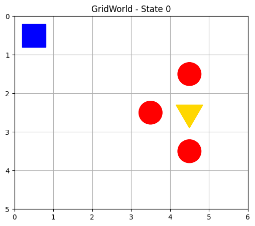
Action: 3, New State: 0, Reward: 0.0
Action: 1, New State: 1, Reward: 0.0
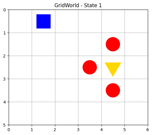
Action: 2, New State: 7, Reward: 0.0
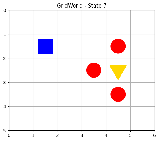
Action: 0, New State: 1, Reward: 0.0
Action: 1, New State: 2, Reward: 0.0
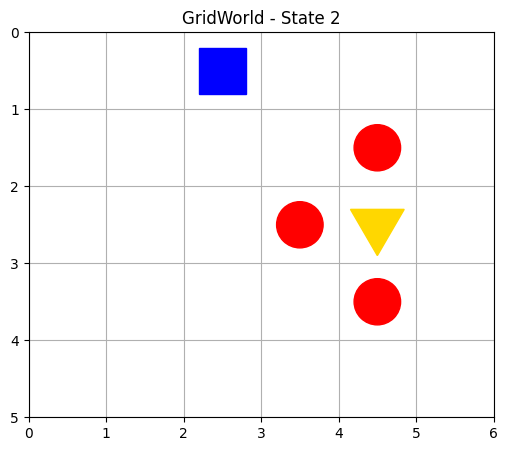
Action: 0, New State: 2, Reward: 0.0
Action: 0, New State: 2, Reward: 0.0
Action: 2, New State: 8, Reward: 0.0
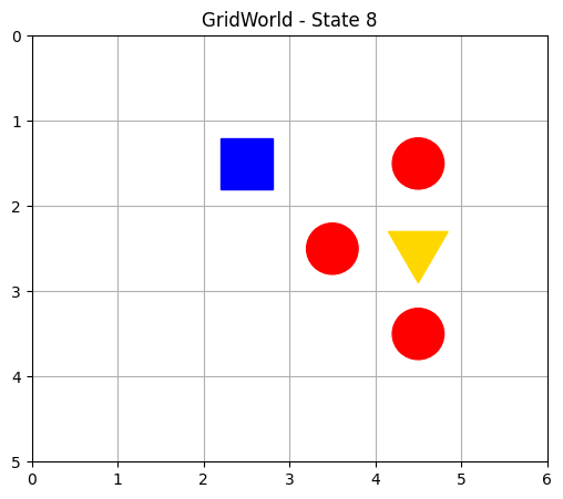
Action: 1, New State: 9, Reward: 0.0
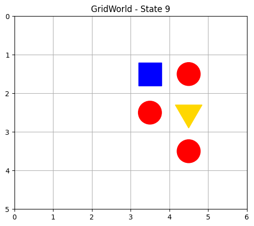
Action: 1, New State: 10, Reward: -1.0
Solving a grid world problem with Q-learning
# agent.py
# Q-Learning Agent for GridWorld
# Adapted from Python Machine Learning, PyTorch Edition (Raschka et al.)

from collections import defaultdict
import numpy as np


class Agent:
    def __init__(
        self, env,
        learning_rate=0.1,
        discount_factor=0.95,
        epsilon_greedy=1.0,
        epsilon_min=0.1,
        epsilon_decay=0.99
    ):
        """
        Q-learning agent
        """
        self.env = env
        self.lr = learning_rate
        self.gamma = discount_factor
        self.epsilon = epsilon_greedy
        self.epsilon_min = epsilon_min
        self.epsilon_decay = epsilon_decay

        # Q-table: maps state to action values
        self.q_table = defaultdict(lambda: np.zeros(self.env.nA))

    def choose_action(self, state):
        """
        Epsilon-greedy action selection
        """
        if np.random.uniform() < self.epsilon:
            return np.random.choice(self.env.nA)  # Explore
        else:
            q_vals = self.q_table[state]
            # Break ties randomly
            best_actions = np.flatnonzero(q_vals == q_vals.max())
            return np.random.choice(best_actions)

    def learn(self, transition):
        """
        Q-Learning update
        """
        s, a, r, next_s, done = transition
        current_q = self.q_table[s][a]

        if done:
            target = r
        else:
            target = r + self.gamma * np.max(self.q_table[next_s])

        self.q_table[s][a] += self.lr * (target - current_q)

        # Decay epsilon (less greedy exploration after agent gradually find the optimal path)
        self._adjust_epsilon()

    def _adjust_epsilon(self):
        if self.epsilon > self.epsilon_min:
            self.epsilon *= self.epsilon_decay
# qlearning.py
# Q-Learning on GridWorld Environment (in previous code block)
from collections import namedtuple
import matplotlib.pyplot as plt
import numpy as np
# For reproducibility
np.random.seed(1)
# Named tuple for transitions
Transition = namedtuple('Transition', ['state', 'action', 'reward', 'next_state', 'done'])
def run_qlearning(agent, env, num_episodes=100, visualize=False):
"""
Run Q-learning over multiple episodes
Returns: history list with (num_moves, final_reward) per episode
"""
history = []
for episode in range(num_episodes):
state, _ = env.reset()
done = False
total_reward, n_moves = 0.0, 0
while not done:
if visualize:
env.render_matplotlib()
action = agent.choose_action(state)
next_state, reward, done, truncated, _ = env.step(action)
# Learning step
agent.learn(Transition(state, action, reward, next_state, done))
state = next_state
total_reward += reward
n_moves += 1
history.append((n_moves, total_reward))
print(f"Episode {episode+1}: Moves = {n_moves}, Reward = {total_reward:.2f}, Epsilon = {agent.epsilon:.3f}")
return history
def plot_learning_history(history):
"""
Plot training history: number of steps and rewards
"""
episodes = np.arange(len(history))
moves = [h[0] for h in history]
rewards = [h[1] for h in history]
plt.figure(figsize=(14, 6))
# Moves plot
plt.subplot(2, 1, 1)
plt.plot(episodes, moves, marker='o')
plt.title("Q-Learning Progress")
plt.ylabel("Number of Moves")
plt.grid(True)
# Rewards plot
plt.subplot(2, 1, 2)
plt.plot(episodes, rewards, drawstyle='steps-post')
plt.xlabel("Episode")
plt.ylabel("Final Reward")
plt.grid(True)
plt.tight_layout()
plt.show()
if __name__ == '__main__':
env = GridWorldEnv(num_rows=5, num_cols=6)
agent = Agent(env)
history = run_qlearning(agent, env, num_episodes=100, visualize=False)
env.close()
plot_learning_history(history)Episode 1: Moves = 10, Reward = -1.00, Epsilon = 0.904
Episode 2: Moves = 60, Reward = -1.00, Epsilon = 0.495
Episode 3: Moves = 18, Reward = -1.00, Epsilon = 0.413
Episode 4: Moves = 28, Reward = -1.00, Epsilon = 0.312
Episode 5: Moves = 6, Reward = -1.00, Epsilon = 0.293
Episode 6: Moves = 48, Reward = -1.00, Epsilon = 0.181
Episode 7: Moves = 43, Reward = -1.00, Epsilon = 0.118
Episode 8: Moves = 149, Reward = -1.00, Epsilon = 0.099
Episode 9: Moves = 13, Reward = -1.00, Epsilon = 0.099
Episode 10: Moves = 135, Reward = -1.00, Epsilon = 0.099
Episode 11: Moves = 173, Reward = -1.00, Epsilon = 0.099
Episode 12: Moves = 42, Reward = -1.00, Epsilon = 0.099
Episode 13: Moves = 13, Reward = -1.00, Epsilon = 0.099
Episode 14: Moves = 427, Reward = 1.00, Epsilon = 0.099
Episode 15: Moves = 50, Reward = -1.00, Epsilon = 0.099
Episode 16: Moves = 264, Reward = -1.00, Epsilon = 0.099
Episode 17: Moves = 43, Reward = -1.00, Epsilon = 0.099
Episode 18: Moves = 115, Reward = -1.00, Epsilon = 0.099
Episode 19: Moves = 57, Reward = 1.00, Epsilon = 0.099
Episode 20: Moves = 12, Reward = -1.00, Epsilon = 0.099
Episode 21: Moves = 37, Reward = -1.00, Epsilon = 0.099
Episode 22: Moves = 92, Reward = 1.00, Epsilon = 0.099
Episode 23: Moves = 17, Reward = -1.00, Epsilon = 0.099
Episode 24: Moves = 149, Reward = -1.00, Epsilon = 0.099
Episode 25: Moves = 66, Reward = 1.00, Epsilon = 0.099
Episode 26: Moves = 125, Reward = 1.00, Epsilon = 0.099
Episode 27: Moves = 74, Reward = -1.00, Epsilon = 0.099
Episode 28: Moves = 17, Reward = 1.00, Epsilon = 0.099
Episode 29: Moves = 293, Reward = 1.00, Epsilon = 0.099
Episode 30: Moves = 83, Reward = 1.00, Epsilon = 0.099
Episode 31: Moves = 27, Reward = -1.00, Epsilon = 0.099
Episode 32: Moves = 40, Reward = -1.00, Epsilon = 0.099
Episode 33: Moves = 15, Reward = 1.00, Epsilon = 0.099
Episode 34: Moves = 23, Reward = 1.00, Epsilon = 0.099
Episode 35: Moves = 43, Reward = 1.00, Epsilon = 0.099
Episode 36: Moves = 10, Reward = 1.00, Epsilon = 0.099
Episode 37: Moves = 12, Reward = 1.00, Epsilon = 0.099
Episode 38: Moves = 8, Reward = 1.00, Epsilon = 0.099
Episode 39: Moves = 12, Reward = 1.00, Epsilon = 0.099
Episode 40: Moves = 10, Reward = 1.00, Epsilon = 0.099
Episode 41: Moves = 8, Reward = 1.00, Epsilon = 0.099
Episode 42: Moves = 10, Reward = 1.00, Epsilon = 0.099
Episode 43: Moves = 9, Reward = 1.00, Epsilon = 0.099
Episode 44: Moves = 8, Reward = 1.00, Epsilon = 0.099
Episode 45: Moves = 8, Reward = 1.00, Epsilon = 0.099
Episode 46: Moves = 10, Reward = 1.00, Epsilon = 0.099
Episode 47: Moves = 7, Reward = -1.00, Epsilon = 0.099
Episode 48: Moves = 11, Reward = 1.00, Epsilon = 0.099
Episode 49: Moves = 12, Reward = 1.00, Epsilon = 0.099
Episode 50: Moves = 8, Reward = 1.00, Epsilon = 0.099
Episode 51: Moves = 11, Reward = 1.00, Epsilon = 0.099
Episode 52: Moves = 8, Reward = 1.00, Epsilon = 0.099
Episode 53: Moves = 10, Reward = 1.00, Epsilon = 0.099
Episode 54: Moves = 8, Reward = 1.00, Epsilon = 0.099
Episode 55: Moves = 8, Reward = 1.00, Epsilon = 0.099
Episode 56: Moves = 8, Reward = 1.00, Epsilon = 0.099
Episode 57: Moves = 8, Reward = 1.00, Epsilon = 0.099
Episode 58: Moves = 8, Reward = 1.00, Epsilon = 0.099
Episode 59: Moves = 9, Reward = 1.00, Epsilon = 0.099
Episode 60: Moves = 11, Reward = 1.00, Epsilon = 0.099
Episode 61: Moves = 10, Reward = 1.00, Epsilon = 0.099
Episode 62: Moves = 8, Reward = 1.00, Epsilon = 0.099
Episode 63: Moves = 8, Reward = 1.00, Epsilon = 0.099
Episode 64: Moves = 8, Reward = 1.00, Epsilon = 0.099
Episode 65: Moves = 9, Reward = 1.00, Epsilon = 0.099
Episode 66: Moves = 8, Reward = 1.00, Epsilon = 0.099
Episode 67: Moves = 10, Reward = 1.00, Epsilon = 0.099
Episode 68: Moves = 8, Reward = 1.00, Epsilon = 0.099
Episode 69: Moves = 8, Reward = 1.00, Epsilon = 0.099
Episode 70: Moves = 10, Reward = 1.00, Epsilon = 0.099
Episode 71: Moves = 5, Reward = -1.00, Epsilon = 0.099
Episode 72: Moves = 8, Reward = 1.00, Epsilon = 0.099
Episode 73: Moves = 8, Reward = 1.00, Epsilon = 0.099
Episode 74: Moves = 12, Reward = 1.00, Epsilon = 0.099
Episode 75: Moves = 8, Reward = 1.00, Epsilon = 0.099
Episode 76: Moves = 8, Reward = 1.00, Epsilon = 0.099
Episode 77: Moves = 8, Reward = 1.00, Epsilon = 0.099
Episode 78: Moves = 9, Reward = 1.00, Epsilon = 0.099
Episode 79: Moves = 8, Reward = 1.00, Epsilon = 0.099
Episode 80: Moves = 11, Reward = 1.00, Epsilon = 0.099
Episode 81: Moves = 8, Reward = 1.00, Epsilon = 0.099
Episode 82: Moves = 8, Reward = 1.00, Epsilon = 0.099
Episode 83: Moves = 10, Reward = 1.00, Epsilon = 0.099
Episode 84: Moves = 8, Reward = 1.00, Epsilon = 0.099
Episode 85: Moves = 12, Reward = 1.00, Epsilon = 0.099
Episode 86: Moves = 10, Reward = 1.00, Epsilon = 0.099
Episode 87: Moves = 8, Reward = 1.00, Epsilon = 0.099
Episode 88: Moves = 10, Reward = 1.00, Epsilon = 0.099
Episode 89: Moves = 9, Reward = 1.00, Epsilon = 0.099
Episode 90: Moves = 8, Reward = 1.00, Epsilon = 0.099
Episode 91: Moves = 10, Reward = 1.00, Epsilon = 0.099
Episode 92: Moves = 9, Reward = 1.00, Epsilon = 0.099
Episode 93: Moves = 10, Reward = 1.00, Epsilon = 0.099
Episode 94: Moves = 8, Reward = 1.00, Epsilon = 0.099
Episode 95: Moves = 8, Reward = 1.00, Epsilon = 0.099
Episode 96: Moves = 8, Reward = 1.00, Epsilon = 0.099
Episode 97: Moves = 8, Reward = 1.00, Epsilon = 0.099
Episode 98: Moves = 8, Reward = 1.00, Epsilon = 0.099
Episode 99: Moves = 8, Reward = 1.00, Epsilon = 0.099
Episode 100: Moves = 9, Reward = 1.00, Epsilon = 0.099
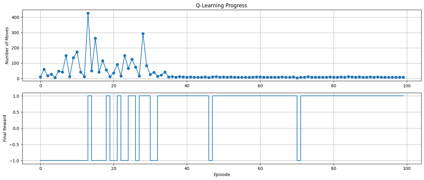
Top plot
The agent is learning how to reach the goal quickly, and over time, it reduces randomness by exploiting known good paths.
Episodes 0–30: High variance — the agent is exploring a lot, sometimes hitting traps, sometimes wandering.
Episodes ~30 onward: Steady drop to ~10–20 moves. This is exactly what you want — it’s a sign the agent has learned the optimal or near-optimal path and is executing it consistently.
Bottom plot
The agent is initially bad (as expected), then improves, and finally consistently reaches the goal without hitting traps.
First 10–15 episodes: Mostly -1 rewards — hitting traps.
Then intermittent 1/-1 rewards: Agent is learning, testing actions, sometimes gets the gold.
After ~30–35: Mostly consistent +1 rewards.
A glance at deep Q-learning
Problems in Tabular Q-learning
Limitations of Tabular Q-learning
Previous example used a discrete state space of size 30.
Q-values were stored in a Python dictionary — feasible for small, finite MDPs.
Problems with Tabular Methods
Large or continuous state spaces make tabular representation intractable.
Infinite or near-infinite states cannot be individually stored.
Sparse visitation: some states might never be visited, making generalization difficult.
Solution: Function Approximation
Replace tabular value functions with parametric functions:
Instead of or , use:
to approximate
to approximate
Here:
: parameters (e.g., weights of a neural network)
: featurized representation of state
Deep Q-Networks (DQN)
A deep Q-network (DQN) is when is modeled using a deep neural network (DNN).
The DNN takes the state (or its features) as input and outputs Q-values for each possible action.
Training DQN
Q-values are updated using the Q-learning update rule (we’ve seen in the lecture). One modification is in the agent’s
choose_action()method, which, in the code of the previous section for Q-learning, was simply accessing the action values stored in a dictionary. Now, this function should be changed to perform a forward pass of the NN model for computing the action values.
Key Insight
DQN allows agents to generalize across unseen states by learning from features.
Makes RL feasible in complex, high-dimensional, or continuous environments where tabular methods fail.
Image(filename='figures/19_10.png', width=600)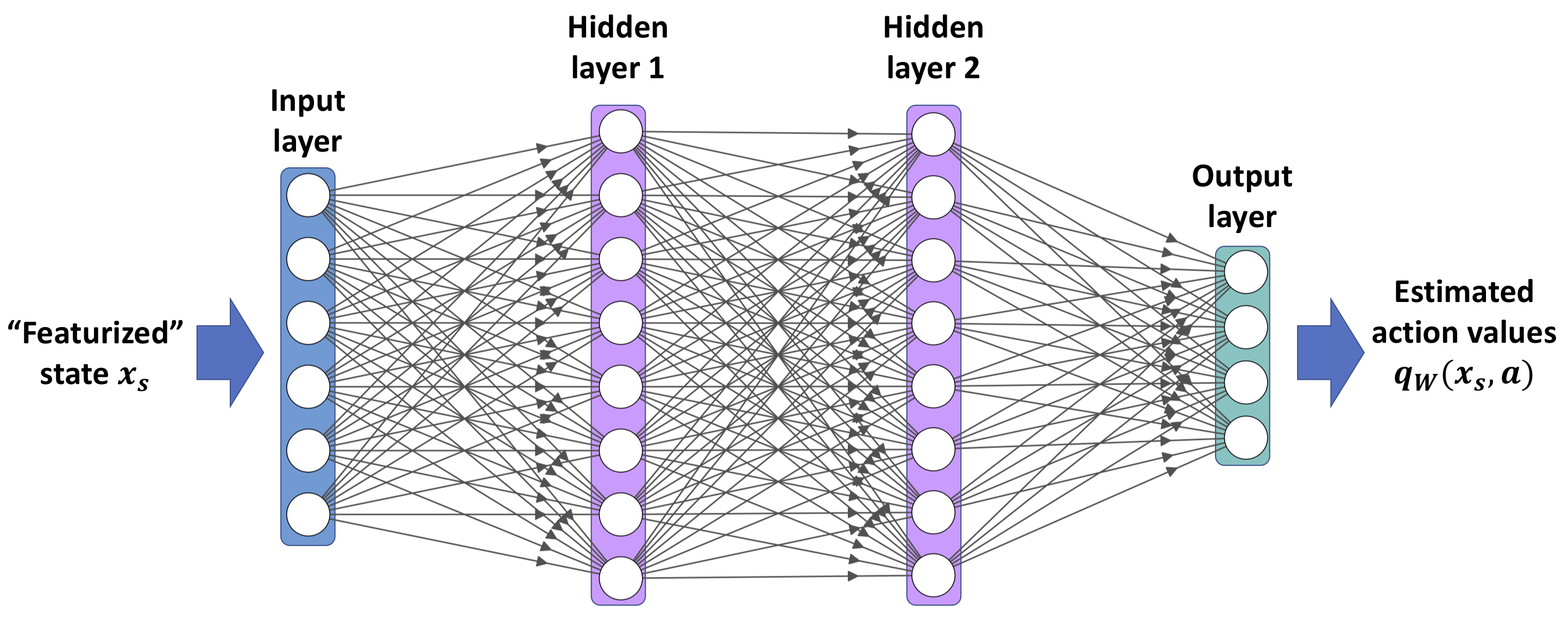
DQN: Replay memory
Challenges with Neural Network Approximation
Interference Between Updates:
In tabular Q-learning, updating a value for a specific state-action pair doesn’t affect others.
With a neural network, updating the weights to fit one state-action pair affects outputs for other states as well.
Changing Distribution of States:
In supervised learning, multiple epochs can be used to train on a fixed dataset.
In Q-learning, the environment is non-stationary: as the agent learns, it visits different states, making older samples less relevant or less likely to reoccur.
Lack of IID Assumption:
Neural networks assume training samples are IID (independent and identically distributed).
In reinforcement learning, transitions are sequential and correlated, violating the IID assumption.
To address these issues, replay memory (also known as experience replay) is introduced.
Transition Storage
As the agent interacts with the environment, it generates transition quintuples:
(These transitions are stored in a finite-sized buffer.)
Buffer Management
The memory buffer is often implemented as a list or queue.
When the buffer is full, the oldest transition is removed to make room for the new one:
memory.pop(0)
Sampling and Training
Instead of training on the most recent transition, the network trains on mini-batches randomly sampled from the buffer
Breaks the correlation between samples.
Helps with better generalization and stability of learning.
Image(filename='figures/19_11.png', width=600)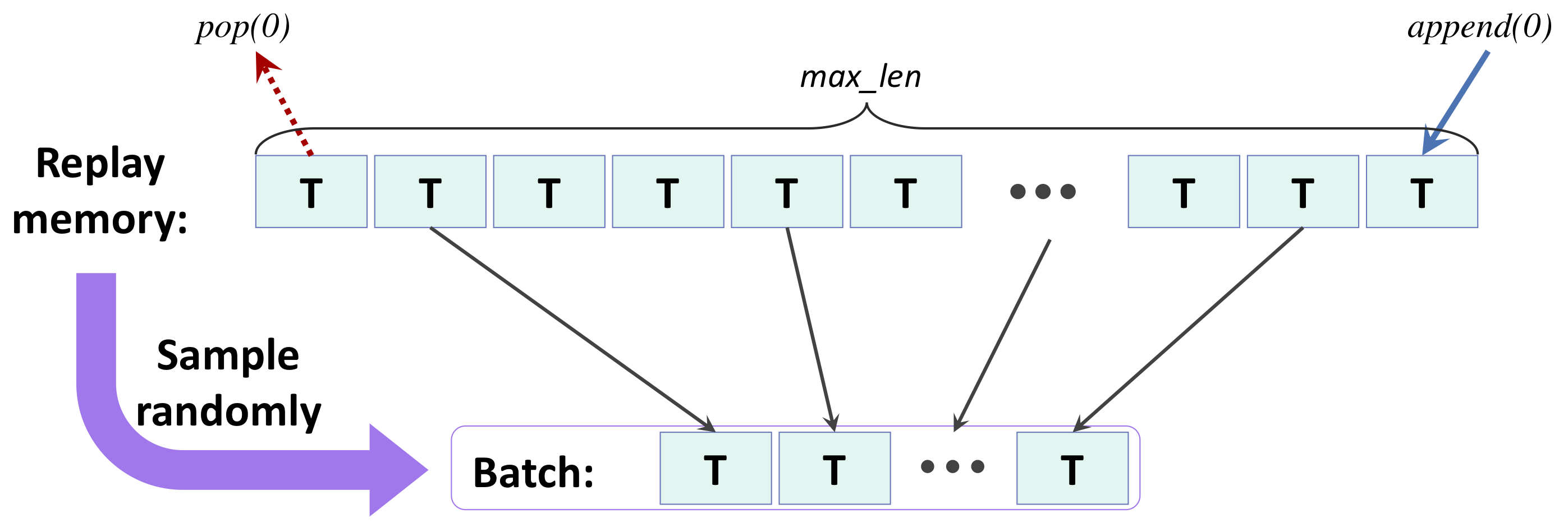
Determining the Target Values for Computing the Loss in DQN
To train a Deep Q-Network (DQN), we need to adapt the update rule from tabular Q-learning to work with neural networks. This involves how we compute the target values used to calculate the loss.
Transition Quintuple
Each stored transition in the replay buffer is of the form:
Where:
: current state features
: action taken
: reward received
: next state features
: boolean indicating if the episode has ended
Dual Forward Passes
To compute the loss, we perform two forward passes through the DQN:
Current state:
Next state:
Here, the notation refers to the vector of Q-values for all possible actions .
Target Value Construction
Using the Q-learning update rule, the target value for the selected action is:
Instead of forming a scalar target, we construct a target Q-value vector that:
Retains the original predicted Q-values for all
Replaces only the entry for action with the computed target
Loss Function
We use a regression objective with:
Predictions:
Target values: vector with the updated entry at index
Loss: Mean Squared Error (MSE) between prediction and target vector
This ensures the loss is non-zero only for the action .
Other entries are unchanged, so gradients will only flow through the relevant output.
Image(filename='figures/19_12.png', width=600)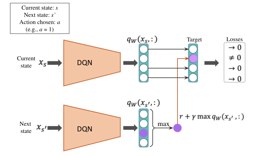
Implementing a deep Q-learning algorithm
# coding: utf-8

# Python Machine Learning, PyTorch Edition by Sebastian Raschka (https://sebastianraschka.com), Yuxi (Hayden) Liu
# (https://www.mlexample.com/) & Vahid Mirjalili (http://vahidmirjalili.com), Packt Publishing Ltd. 2021
#
# Code Repository: https://github.com
#
# Code License: MIT License (https://github.com/ /LICENSE.txt)

#################################################################################
# Chapter 19 - Reinforcement Learning for Decision Making in Complex Environments
#################################################################################

# Script: carpole/main.py

import gym
import numpy as np
import torch
import torch.nn as nn
import random
import matplotlib.pyplot as plt
from collections import namedtuple
from collections import deque

np.random.seed(1)
torch.manual_seed(1)

Transition = namedtuple(
    'Transition', ('state', 'action', 'reward',
                   'next_state', 'done'))


class DQNAgent:
    def __init__(
            self, env, discount_factor=0.95,
            epsilon_greedy=1.0, epsilon_min=0.01,
            epsilon_decay=0.995, learning_rate=1e-3,
            max_memory_size=2000):
        self.env = env
        self.state_size = env.observation_space.shape[0]
        self.action_size = env.action_space.n

        self.memory = deque(maxlen=max_memory_size)

        self.gamma = discount_factor
        self.epsilon = epsilon_greedy
        self.epsilon_min = epsilon_min
        self.epsilon_decay = epsilon_decay
        self.lr = learning_rate
        self._build_nn_model()

    def _build_nn_model(self):
        self.model = nn.Sequential(nn.Linear(self.state_size, 256),
                                   nn.ReLU(),
                                   nn.Linear(256, 128),
                                   nn.ReLU(),
                                   nn.Linear(128, 64),
                                   nn.ReLU(),
                                   nn.Linear(64, self.action_size))

        self.loss_fn = nn.MSELoss()
        self.optimizer = torch.optim.Adam(
            self.model.parameters(), self.lr)

    def remember(self, transition):
        self.memory.append(transition)

    def choose_action(self, state):
        if np.random.rand() <= self.epsilon:
            return np.random.choice(self.action_size)
        with torch.no_grad():
            q_values = self.model(torch.tensor(state, dtype=torch.float32))[0]
        return torch.argmax(q_values).item()  # returns action

    def _learn(self, batch_samples):
        batch_states, batch_targets = [], []
        for transition in batch_samples:
            s, a, r, next_s, done = transition

            with torch.no_grad():
                if done:
                    target = r
                else:
                    pred = self.model(torch.tensor(next_s, dtype=torch.float32))[0]
                    target = r + self.gamma * pred.max()

                target_all = self.model(torch.tensor(s, dtype=torch.float32))[0]
                target_all[a] = target

            batch_states.append(s.flatten())
            batch_targets.append(target_all)
            self._adjust_epsilon()

        self.optimizer.zero_grad()
        pred = self.model(torch.tensor(batch_states, dtype=torch.float32))

        loss = self.loss_fn(pred, torch.stack(batch_targets))
        loss.backward()
        self.optimizer.step()

        return loss.item()

    def _adjust_epsilon(self):
        if self.epsilon > self.epsilon_min:
            self.epsilon *= self.epsilon_decay

    def replay(self, batch_size):
        samples = random.sample(self.memory, batch_size)
        return self._learn(samples)


def plot_learning_history(history):
    fig = plt.figure(1, figsize=(14, 5))
    ax = fig.add_subplot(1, 1, 1)
    episodes = np.arange(len(history)) + 1
    plt.plot(episodes, history, lw=4,
             marker='o', markersize=10)
    ax.tick_params(axis='both', which='major', labelsize=15)
    plt.xlabel('Episodes', size=20)
    plt.ylabel('# Total Rewards', size=20)
    plt.show()


# General settings
EPISODES = 200
batch_size = 32
init_replay_memory_size = 500

if __name__ == '__main__':
    env = gym.make('CartPole-v1')
    agent = DQNAgent(env)
    state = env.reset()
    state = np.reshape(state, [1, agent.state_size])

    # Filling up the replay-memory
    for i in range(init_replay_memory_size):
        action = agent.choose_action(state)
        next_state, reward, done, _ = env.step(action)
        next_state = np.reshape(next_state, [1, agent.state_size])
        agent.remember(Transition(state, action, reward,
                                  next_state, done))
        if done:
            state = env.reset()
            state = np.reshape(state, [1, agent.state_size])
        else:
            state = next_state

    total_rewards, losses = [], []
    for e in range(EPISODES):
        state = env.reset()
        if e % 10 == 0:
            env.render()
        state = np.reshape(state, [1, agent.state_size])
        for i in range(500):
            action = agent.choose_action(state)
            next_state, reward, done, _ = env.step(action)
            next_state = np.reshape(next_state, [1, agent.state_size])
            agent.remember(Transition(state, action, reward,
                                      next_state, done))
            state = next_state
            if e % 10 == 0:
                env.render()
            if done:
                total_rewards.append(i)
                print(f'Episode: {e}/{EPISODES}, Total reward: {i}')
                break
            loss = agent.replay(batch_size)
            losses.append(loss)
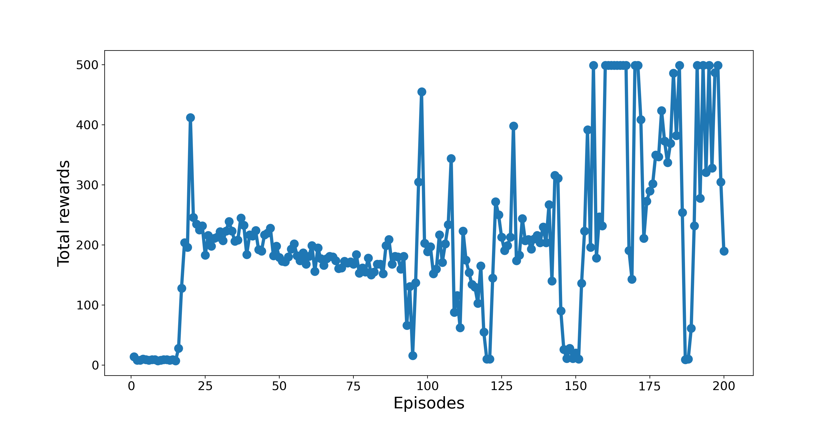
    plot_learning_history(total_rewards)
Image(filename='figures/19_13.png', width=600)