Neural Networks: Theory & Fundamentals¶

From affine neurons to a complete NumPy backpropagation implementation

This notebook follows the lecture notation exactly: a mini-batch $\mathbf{X}\in\mathbb{R}^{B\times D}$ passes through a hidden layer of width $H$ and produces $K$ class probabilities.

Learning Objectives¶

By the end of this notebook, you will be able to:

Trace tensor shapes through an MLP forward pass
Explain why nonlinear hidden features solve problems that a linear model cannot
Implement stable softmax and cross-entropy
Derive and verify backpropagation with finite differences
Train a two-layer neural network using only NumPy
Diagnose the effects of learning rate and regularization from training curves

1. Setup and Locked Notation¶

We use:

$B$ : mini-batch size
$D$ : number of input features
$H$ : hidden width
$K$ : number of output classes
$\mathbf{X}:(B,D)$ , $\mathbf{W}^{(1)}:(D,H)$ , $\mathbf{W}^{(2)}:(H,K)$

import warnings

import matplotlib.pyplot as plt
import numpy as np
from sklearn.datasets import make_moons
from sklearn.exceptions import ConvergenceWarning
from sklearn.linear_model import LogisticRegression
from sklearn.metrics import accuracy_score
from sklearn.model_selection import train_test_split
from sklearn.neural_network import MLPClassifier
from sklearn.pipeline import make_pipeline
from sklearn.preprocessing import StandardScaler

warnings.filterwarnings("ignore", category=ConvergenceWarning)
np.set_printoptions(precision=4, suppress=True)
plt.style.use("seaborn-v0_8-whitegrid")
RANDOM_STATE = 42
print("Imports complete; random state =", RANDOM_STATE)

Matplotlib is building the font cache; this may take a moment.

Imports complete; random state = 42

def stable_softmax(logits):
    shifted = logits - logits.max(axis=1, keepdims=True)
    exp_scores = np.exp(shifted)
    return exp_scores / exp_scores.sum(axis=1, keepdims=True)

rng = np.random.default_rng(RANDOM_STATE)
B, D, H, K = 4, 3, 5, 2
X_demo = rng.normal(size=(B, D))
W1_demo = rng.normal(scale=np.sqrt(2 / D), size=(D, H))
b1_demo = np.zeros(H)
W2_demo = rng.normal(scale=np.sqrt(2 / H), size=(H, K))
b2_demo = np.zeros(K)

Z1_demo = X_demo @ W1_demo + b1_demo
A1_demo = np.maximum(0, Z1_demo)
Z2_demo = A1_demo @ W2_demo + b2_demo
P_demo = stable_softmax(Z2_demo)

for name, array in [("X", X_demo), ("Z1", Z1_demo), ("A1", A1_demo), ("Z2", Z2_demo), ("P", P_demo)]:
    print(f"{name:>2}: shape={array.shape}")
print("Probability row sums:", P_demo.sum(axis=1))

 X: shape=(4, 3)
Z1: shape=(4, 5)
A1: shape=(4, 5)
Z2: shape=(4, 2)
 P: shape=(4, 2)
Probability row sums: [1. 1. 1. 1.]

The inner dimensions of every matrix product must agree. Bias vectors broadcast across the batch dimension. Softmax preserves the $(B,K)$ shape and normalizes each row.

2. Activations Create Nonlinear Features¶

Stacking affine transformations without an activation still produces one affine transformation. An activation changes the function class by bending the representation between layers.

z = np.linspace(-5, 5, 600)
sigmoid = 1 / (1 + np.exp(-z))
tanh = np.tanh(z)
relu = np.maximum(0, z)

fig, axes = plt.subplots(1, 2, figsize=(11, 4))
axes[0].plot(z, sigmoid, label="sigmoid")
axes[0].plot(z, tanh, label="tanh")
axes[0].plot(z, relu, label="ReLU")
axes[0].set(title="Activation functions", xlabel="z", ylabel="activation")
axes[0].legend()

axes[1].plot(z, sigmoid * (1 - sigmoid), label="sigmoid′")
axes[1].plot(z, 1 - tanh**2, label="tanh′")
axes[1].plot(z, (z > 0).astype(float), label="ReLU′")
axes[1].set(title="Local derivatives", xlabel="z", ylabel="derivative", ylim=(-0.05, 1.05))
axes[1].legend()
plt.tight_layout()
plt.show()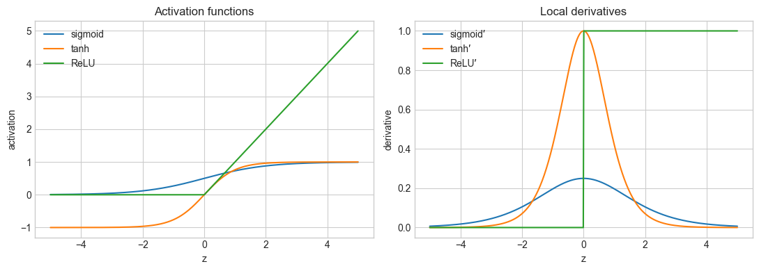

A concrete representation: XOR¶

For binary inputs, two ReLU hidden features solve XOR exactly:

h_1=\operatorname{ReLU}(x_1+x_2),\qquad h_2=\operatorname{ReLU}(x_1+x_2-1),

(1)

\hat y=h_1-2h_2.

(2)

The hidden layer changes the representation so that a linear output can solve the transformed problem.

X_xor = np.array([[0, 0], [0, 1], [1, 0], [1, 1]], dtype=float)
h1 = np.maximum(0, X_xor.sum(axis=1))
h2 = np.maximum(0, X_xor.sum(axis=1) - 1)
y_xor = h1 - 2 * h2
print(np.c_[X_xor, h1, h2, y_xor])

[[0. 0. 0. 0. 0.]
 [0. 1. 1. 0. 1.]
 [1. 0. 1. 0. 1.]
 [1. 1. 2. 1. 0.]]

3. Empirical Checkpoint: Linear Model vs MLP¶

The two-moons dataset is deliberately nonlinear. Both models receive the same standardized features; only their representational capacity differs.

X, y = make_moons(n_samples=600, noise=0.22, random_state=RANDOM_STATE)
X_train, X_test, y_train, y_test = train_test_split(
    X, y, test_size=0.30, stratify=y, random_state=RANDOM_STATE
)

linear_model = make_pipeline(
    StandardScaler(),
    LogisticRegression(C=10, max_iter=2000, random_state=RANDOM_STATE),
)
mlp_model = make_pipeline(
    StandardScaler(),
    MLPClassifier(
        hidden_layer_sizes=(16,), activation="relu", solver="adam",
        alpha=1e-4, learning_rate_init=0.01, max_iter=600,
        early_stopping=True, n_iter_no_change=35, random_state=RANDOM_STATE,
    ),
)

for model in (linear_model, mlp_model):
    model.fit(X_train, y_train)

print(f"Logistic regression test accuracy: {linear_model.score(X_test, y_test):.3f}")
print(f"MLP test accuracy:                 {mlp_model.score(X_test, y_test):.3f}")

Logistic regression test accuracy: 0.861
MLP test accuracy:                 0.894

def plot_decision_boundary(ax, model, X, y, title):
    pad = 0.6
    x1 = np.linspace(X[:, 0].min() - pad, X[:, 0].max() + pad, 350)
    x2 = np.linspace(X[:, 1].min() - pad, X[:, 1].max() + pad, 350)
    xx1, xx2 = np.meshgrid(x1, x2)
    grid = np.c_[xx1.ravel(), xx2.ravel()]
    prob = model.predict_proba(grid)[:, 1].reshape(xx1.shape)
    ax.contourf(xx1, xx2, prob, levels=np.linspace(0, 1, 12), cmap="RdBu_r", alpha=0.55)
    ax.contour(xx1, xx2, prob, levels=[0.5], colors="black", linewidths=2)
    ax.scatter(X[:, 0], X[:, 1], c=y, cmap="RdBu_r", edgecolor="white", s=28)
    ax.set(title=title, xlabel="$x_1$", ylabel="$x_2$")

fig, axes = plt.subplots(1, 2, figsize=(12, 4.6))
plot_decision_boundary(axes[0], linear_model, X_test, y_test, "Logistic regression: one linear boundary")
plot_decision_boundary(axes[1], mlp_model, X_test, y_test, "MLP: learned nonlinear boundary")
plt.tight_layout()
plt.show()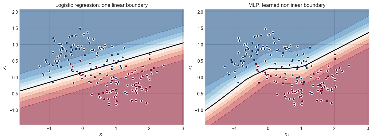

4. Stable Softmax and Cross-Entropy¶

For one-hot targets $\mathbf{Y}$ , the averaged cross-entropy is

\mathcal{L}=-\frac{1}{B}\sum_{i=1}^{B}\sum_{k=1}^{K}y_{ik}\log(p_{ik}+\varepsilon).

(3)

Subtracting each row’s maximum before exponentiation avoids overflow without changing softmax probabilities.

def cross_entropy(probabilities, y_true):
    return -np.log(probabilities[np.arange(len(y_true)), y_true] + 1e-12).mean()

extreme_logits = np.array([[1000.0, 1001.0, 999.0], [-1000.0, -999.0, -1002.0]])
probabilities = stable_softmax(extreme_logits)
print("Stable probabilities:\n", probabilities)
print("Row sums:", probabilities.sum(axis=1))
print("Cross-entropy:", cross_entropy(probabilities, np.array([1, 1])))

Stable probabilities:
 [[0.24472847 0.66524096 0.09003057]
 [0.25949646 0.70538451 0.03511903]]
Row sums: [1. 1.]
Cross-entropy: 0.378309090604823

5. Backpropagation in Matrix Form¶

For a ReLU hidden layer and softmax output:

\mathbf{G}^{(2)}=(\mathbf{P}-\mathbf{Y})/B,

(4)

\nabla_{\mathbf{W}^{(2)}}\mathcal{L}=\mathbf{A}^{(1)\top}\mathbf{G}^{(2)},

(5)

\mathbf{G}^{(1)}=(\mathbf{G}^{(2)}\mathbf{W}^{(2)\top})\odot\mathbf{1}[\mathbf{Z}^{(1)}>0],

(6)

\nabla_{\mathbf{W}^{(1)}}\mathcal{L}=\mathbf{X}^{\top}\mathbf{G}^{(1)}.

(7)

Bias gradients sum the corresponding $\mathbf{G}$ over the batch axis.

def forward(X, params):
    Z1 = X @ params["W1"] + params["b1"]
    A1 = np.maximum(0, Z1)
    Z2 = A1 @ params["W2"] + params["b2"]
    P = stable_softmax(Z2)
    return P, {"X": X, "Z1": Z1, "A1": A1, "P": P}

def backward(y, params, cache, l2=0.0):
    B = len(y)
    Y = np.eye(params["b2"].size)[y]
    G2 = (cache["P"] - Y) / B
    dW2 = cache["A1"].T @ G2 + l2 * params["W2"]
    db2 = G2.sum(axis=0)
    G1 = (G2 @ params["W2"].T) * (cache["Z1"] > 0)
    dW1 = cache["X"].T @ G1 + l2 * params["W1"]
    db1 = G1.sum(axis=0)
    return {"W1": dW1, "b1": db1, "W2": dW2, "b2": db2}

params_demo = {"W1": W1_demo.copy(), "b1": b1_demo.copy(), "W2": W2_demo.copy(), "b2": b2_demo.copy()}
y_demo = np.array([0, 1, 1, 0])
P, cache = forward(X_demo, params_demo)
grads = backward(y_demo, params_demo, cache)
for name in params_demo:
    print(f"{name}: parameter {params_demo[name].shape}, gradient {grads[name].shape}")

W1: parameter (3, 5), gradient (3, 5)
b1: parameter (5,), gradient (5,)
W2: parameter (5, 2), gradient (5, 2)
b2: parameter (2,), gradient (2,)

Gradient checking¶

Backpropagation is easy to implement incorrectly. A centered finite difference provides an independent numerical check:

g_j^{num}=\frac{\mathcal{L}(\theta_j+\epsilon)-\mathcal{L}(\theta_j-\epsilon)}{2\epsilon}.

(8)

def gradient_check(X, y, params, epsilon=1e-5):
    P, cache = forward(X, params)
    analytic = backward(y, params, cache)
    numerical = {name: np.zeros_like(value) for name, value in params.items()}

    for name, value in params.items():
        for index in np.ndindex(value.shape):
            original = value[index]
            value[index] = original + epsilon
            plus = cross_entropy(forward(X, params)[0], y)
            value[index] = original - epsilon
            minus = cross_entropy(forward(X, params)[0], y)
            value[index] = original
            numerical[name][index] = (plus - minus) / (2 * epsilon)

    a = np.concatenate([analytic[name].ravel() for name in params])
    n = np.concatenate([numerical[name].ravel() for name in params])
    return np.linalg.norm(a - n) / (np.linalg.norm(a) + np.linalg.norm(n) + 1e-12)

tiny_rng = np.random.default_rng(7)
tiny_params = {
    "W1": tiny_rng.normal(0, 0.2, size=(3, 4)), "b1": np.full(4, 0.05),
    "W2": tiny_rng.normal(0, 0.2, size=(4, 2)), "b2": np.zeros(2),
}
relative_error = gradient_check(X_demo, y_demo, tiny_params)
print(f"Relative gradient error: {relative_error:.2e}")
assert relative_error < 1e-6

Relative gradient error: 4.59e-11

6. A Complete NumPy MLP¶

The implementation below adds He initialization, mini-batch updates, $L_2$ regularization, deterministic shuffling, and training-history capture. Frameworks automate these pieces, but the underlying operations are the same.

class NumPyMLP:
    def __init__(self, n_features, n_hidden, n_classes, learning_rate=0.05, l2=1e-4, random_state=42):
        self.learning_rate = learning_rate
        self.l2 = l2
        self.rng = np.random.default_rng(random_state)
        self.params = {
            "W1": self.rng.normal(0, np.sqrt(2 / n_features), size=(n_features, n_hidden)),
            "b1": np.zeros(n_hidden),
            "W2": self.rng.normal(0, np.sqrt(2 / n_hidden), size=(n_hidden, n_classes)),
            "b2": np.zeros(n_classes),
        }
        self.history = {"loss": [], "accuracy": []}

    def fit(self, X, y, epochs=800, batch_size=64):
        for _ in range(epochs):
            order = self.rng.permutation(len(X))
            for start in range(0, len(X), batch_size):
                idx = order[start:start + batch_size]
                P, cache = forward(X[idx], self.params)
                grads = backward(y[idx], self.params, cache, l2=self.l2)
                for name in self.params:
                    self.params[name] -= self.learning_rate * grads[name]

            P_all, _ = forward(X, self.params)
            data_loss = cross_entropy(P_all, y)
            penalty = 0.5 * self.l2 * (np.sum(self.params["W1"]**2) + np.sum(self.params["W2"]**2))
            self.history["loss"].append(data_loss + penalty)
            self.history["accuracy"].append(accuracy_score(y, P_all.argmax(axis=1)))
        return self

    def predict_proba(self, X):
        return forward(X, self.params)[0]

    def predict(self, X):
        return self.predict_proba(X).argmax(axis=1)

scaler = StandardScaler()
X_train_s = scaler.fit_transform(X_train)
X_test_s = scaler.transform(X_test)

numpy_mlp = NumPyMLP(2, 16, 2, learning_rate=0.05, l2=1e-4, random_state=RANDOM_STATE)
numpy_mlp.fit(X_train_s, y_train, epochs=800, batch_size=64)

print(f"Final training accuracy: {numpy_mlp.history['accuracy'][-1]:.3f}")
print(f"Test accuracy:           {accuracy_score(y_test, numpy_mlp.predict(X_test_s)):.3f}")
print("Parameter count:", sum(value.size for value in numpy_mlp.params.values()))

Final training accuracy: 0.957
Test accuracy:           0.961
Parameter count: 82

fig, axes = plt.subplots(1, 2, figsize=(12, 4.5))
axes[0].plot(numpy_mlp.history["loss"], label="training loss")
axes[0].set(title="NumPy MLP optimization", xlabel="epoch", ylabel="cross-entropy + penalty")
axes[0].legend()

class ScaledNumPyMLP:
    def __init__(self, scaler, model):
        self.scaler, self.model = scaler, model
    def predict_proba(self, X):
        return self.model.predict_proba(self.scaler.transform(X))

plot_decision_boundary(axes[1], ScaledNumPyMLP(scaler, numpy_mlp), X_test, y_test, "NumPy MLP decision boundary")
plt.tight_layout()
plt.show()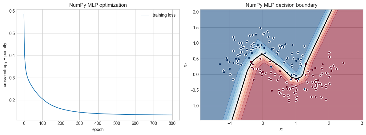

7. Learning-Rate Experiment¶

Everything except the learning rate is held fixed. Compare both convergence speed and stability; the final loss alone does not tell the whole story.

rates = [0.005, 0.05, 0.5]
fig, ax = plt.subplots(figsize=(8, 4.5))
rate_results = []
for rate in rates:
    model = NumPyMLP(2, 16, 2, learning_rate=rate, l2=1e-4, random_state=RANDOM_STATE)
    model.fit(X_train_s, y_train, epochs=300, batch_size=64)
    test_acc = accuracy_score(y_test, model.predict(X_test_s))
    rate_results.append((rate, model.history["loss"][-1], test_acc))
    ax.plot(model.history["loss"], label=f"η={rate:g}")

ax.set(title="Learning rate changes training dynamics", xlabel="epoch", ylabel="training objective")
ax.set_yscale("log")
ax.legend()
plt.tight_layout()
plt.show()

for rate, loss, acc in rate_results:
    print(f"η={rate:<5g} final loss={loss:.4f}, test accuracy={acc:.3f}")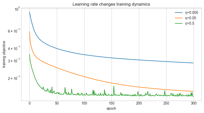

η=0.005 final loss=0.2816, test accuracy=0.889
η=0.05  final loss=0.1455, test accuracy=0.950
η=0.5   final loss=0.1294, test accuracy=0.961

8. Validation Curves and Early Stopping¶

The scikit-learn MLP reserved part of the training data for validation. Early stopping keeps training from continuing after validation performance stops improving.

trained_mlp = mlp_model.named_steps["mlpclassifier"]
fig, axes = plt.subplots(1, 2, figsize=(11, 4))
axes[0].plot(trained_mlp.loss_curve_)
axes[0].set(title="Training loss", xlabel="iteration", ylabel="loss")
if hasattr(trained_mlp, "validation_scores_") and trained_mlp.validation_scores_ is not None:
    axes[1].plot(trained_mlp.validation_scores_)
    axes[1].axvline(np.argmax(trained_mlp.validation_scores_), color="tab:red", linestyle="--", label="best")
    axes[1].legend()
axes[1].set(title="Held-out validation accuracy", xlabel="iteration", ylabel="accuracy")
plt.tight_layout()
plt.show()
print(f"Stopped after {trained_mlp.n_iter_} iterations; best validation score = {trained_mlp.best_validation_score_:.3f}")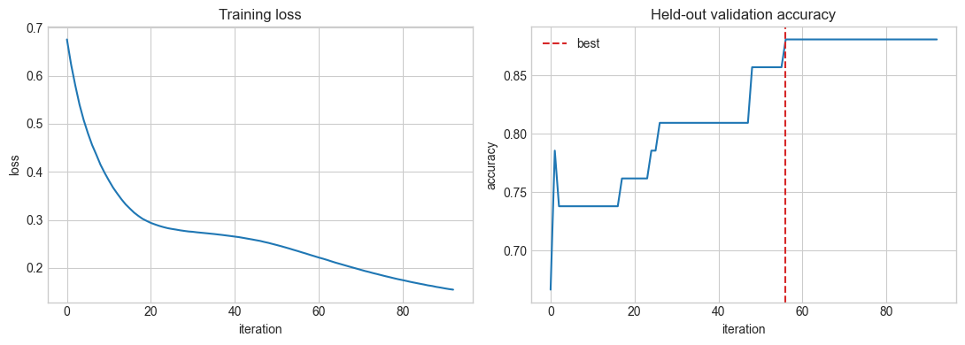

Stopped after 93 iterations; best validation score = 0.881

9. Summary¶

A hidden activation prevents stacked affine layers from collapsing into one linear model.
Stable softmax and cross-entropy turn logits into a well-behaved multiclass objective.
Backpropagation is the chain rule applied efficiently in reverse.
Gradient checking validates the implementation before expensive training.
He initialization, standardized inputs, learning rate, and regularization all affect trainability.
Curves and error patterns are evidence; defaults are only starting points.

Exercises¶

Replace ReLU with tanh in NumPyMLP; update both the forward and backward functions.
Add momentum to the optimizer and compare convergence at the three learning rates.
Sweep hidden width over $H\in\{2,4,16,64\}$ and plot train/test accuracy.
Make the two-moons noise level larger. Which intervention helps: width, regularization, or more data?

References¶

Rumelhart, D. E., Hinton, G. E., & Williams, R. J. (1986). Learning representations by back-propagating errors. Nature, 323, 533–536. https://www.nature.com/articles/323533a0
Glorot, X., & Bengio, Y. (2010). Understanding the difficulty of training deep feedforward neural networks. AISTATS. https://proceedings.mlr.press/v9/glorot10a.html
He, K., Zhang, X., Ren, S., & Sun, J. (2015). Delving Deep into Rectifiers. ICCV. https://openaccess.thecvf.com/content_iccv_2015/html/He_Delving_Deep_into_ICCV_2015_paper.html
Raschka, S., & Mirjalili, V. (2022). Machine Learning with PyTorch and Scikit-Learn, Chapters 11–12.
Goodfellow, I., Bengio, Y., & Courville, A. (2016). Deep Learning, Chapters 6–8. https://www.deeplearningbook.org/