Chapter 14 - CNN¶

from IPython.display import Image
%matplotlib inline

Convolution Layer¶

1D convolution output¶

import torch
import numpy as np

print('PyTorch version:', torch.__version__)
print('NumPy version: ', np.__version__)

PyTorch version: 2.0.0
NumPy version:  1.22.2

def conv1d(x, w, p=0, s=1):
    w_rot = np.array(w[::-1])
    x_padded = np.array(x)
    if p > 0:
        zero_pad = np.zeros(shape=p)
        x_padded = np.concatenate(
            [zero_pad, x_padded, zero_pad])
    res = []
    for i in range(0, int((len(x_padded) - len(w_rot))) + 1, s):
        res.append(np.sum(
            x_padded[i:i+w_rot.shape[0]] * w_rot))
    return np.array(res)


## Testing:
x = [1, 3, 2, 4, 5, 6, 1, 3]
w = [1, 0, 3, 1, 2]

print('Conv1d Implementation:',
      conv1d(x, w, p=2, s=1))

print('Numpy Results:',
      np.convolve(x, w, mode='same'))

Conv1d Implementation: [ 5. 14. 16. 26. 24. 34. 19. 22.]
Numpy Results: [ 5 14 16 26 24 34 19 22]

2D convolution output¶

import scipy.signal


def conv2d(X, W, p=(0, 0), s=(1, 1)):
    W_rot = np.array(W)[::-1,::-1]
    X_orig = np.array(X)
    n1 = X_orig.shape[0] + 2*p[0]
    n2 = X_orig.shape[1] + 2*p[1]
    X_padded = np.zeros(shape=(n1, n2))
    X_padded[p[0]:p[0]+X_orig.shape[0],
    p[1]:p[1]+X_orig.shape[1]] = X_orig

    res = []
    for i in range(0, int((X_padded.shape[0] - 
                           W_rot.shape[0])/s[0])+1, s[0]):
        res.append([])
        for j in range(0, int((X_padded.shape[1] - 
                               W_rot.shape[1])/s[1])+1, s[1]):
            X_sub = X_padded[i:i+W_rot.shape[0],
                             j:j+W_rot.shape[1]]
            res[-1].append(np.sum(X_sub * W_rot))
    return(np.array(res))

X = [[1, 3, 2, 4], [5, 6, 1, 3], [1, 2, 0, 2], [3, 4, 3, 2]]
W = [[1, 0, 3], [1, 2, 1], [0, 1, 1]]

print('Conv2d Implementation:\n',
    conv2d(X, W, p=(1, 1), s=(1, 1)))


print('SciPy Results:\n',
    scipy.signal.convolve2d(X, W, mode='same'))

Conv2d Implementation:
 [[11. 25. 32. 13.]
 [19. 25. 24. 13.]
 [13. 28. 25. 17.]
 [11. 17. 14.  9.]]
SciPy Results:
 [[11 25 32 13]
 [19 25 24 13]
 [13 28 25 17]
 [11 17 14  9]]

Implementing a CNN¶

Overview¶

channels = $N_1 \times N_2$ matrices: input matrices to a convolutional layer
Conventional implementations of convolutional layers expect a rank-3 tensor representation as an input, for example, a three-dimensional array, $\boldsymbol{X}_{N_1 \times N_2 \times C_{i n}}$
- $C_{in}$ : number of input channels
  - RGB color mode: $C_{in}=3$
  - Grayscale (pixel intensity) mode: $C_{in}=1$

Reading an image file

When we work with images, we can read images into NumPy arrays using the uint8 (unsigned 8-bit integer) data type to reduce memory usage compared to 16-bit, 32-bit, or 64-bit integer types, for example.

Unsigned 8-bit integers take values in the range [0, 255], which are sufficient to store the pixel information in RGB images, which also take values in the same range.

import torch
from torchvision.io import read_image

img = read_image('example-image.png') 

print('Image shape:', img.shape)
print('Number of channels:', img.shape[0])
print('Image data type:', img.dtype)
print(img[:, 100:102, 100:102])

Image shape: torch.Size([3, 252, 221])
Number of channels: 3
Image data type: torch.uint8
tensor([[[179, 182],
         [180, 182]],

        [[134, 136],
         [135, 137]],

        [[110, 112],
         [111, 113]]], dtype=torch.uint8)

Formula¶

Recall the multilayer NNs

$\boldsymbol{Z}=\boldsymbol{W} * \boldsymbol{X}+\boldsymbol{b}$ = pre-activations in CNN = net inputs
- $\boldsymbol{W}$ : the weight matrix connecting the pixel inputs to each hidden unit
- $\boldsymbol{X}$ : input matrix representing the pixels in a height × width arrangement
$\boldsymbol{A}=\sigma(\boldsymbol{Z})$ = feature map in CNN= activation of a hidden unit
- $\sigma$ = activation function
- Usually, a convolutional layer of a CNN has more than one feature map.

The total pre-activation result is computed in the following formula:

$C_{in}$ = number of input channels

If we use multiple feature maps,

kernel (4D-tensor) = width $\times$ height $\times C_{in} \times C_{\text {out}}$
$C_{out}$ = number of output feature maps

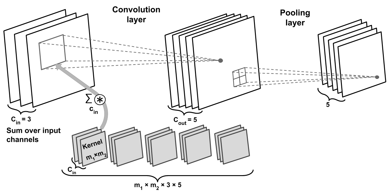
Example illustration¶

input channels: 3
output channels: 5
kernel tensor: 4D (grey blocks in the figure)
- each kernel matrix: $m_1 \times m_2$ ,
- number of kernels matrix: 3, for 3 input channels
- number of kernels: 5, for 5 output feature maps
pooling layer: subsampling the feature maps

Regularizing an NN with L2 regularization and dropout¶

L2 Regularization¶

Choosing the size of a network, whether we are dealing with a traditional (fully connected) NN or a CNN, has always been a challenging problem. For instance, the size of a weight matrix and the number of layers need to be tuned to achieve a reasonably good performance.

Small networks $\rightarrow$ small number of parameters $\rightarrow$ low capacity $\rightarrow$ underfit $\rightarrow$ poor performance

When we deal with real-world machine learning problems, we do not know how large the network should be a priori. In practice, we want to choose a capacity that is slightly larger than necessary to do well on the training dataset. Then, to prevent overfitting by regularization schemes.

import torch.nn as nn


loss_func = nn.BCELoss()
loss = loss_func(torch.tensor([0.9]), torch.tensor([1.0]))
l2_lambda = 0.001

conv_layer = nn.Conv2d(in_channels=3, out_channels=5, kernel_size=5)
l2_penalty = l2_lambda * sum([(p**2).sum() for p in conv_layer.parameters()])
loss_with_penalty = loss + l2_penalty
loss_with_penalty

tensor(0.1069, grad_fn=<AddBackward0>)


linear_layer = nn.Linear(10, 16)
l2_penalty = l2_lambda * sum([(p**2).sum() for p in linear_layer.parameters()])
loss_with_penalty = loss + l2_penalty
loss_with_penalty

tensor(0.1108, grad_fn=<AddBackward0>)

Dropout¶

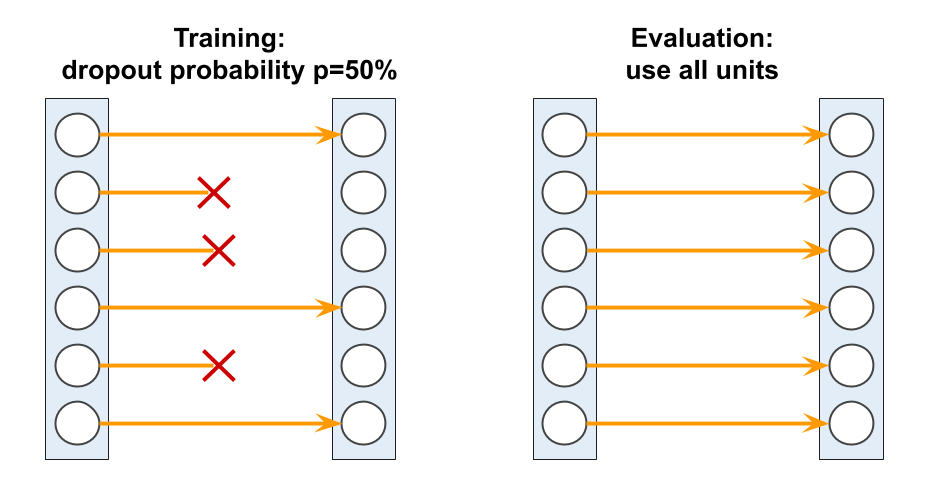
Dropout is usually applied to the hidden units of higher layers and works as follows:

During the training phase of an NN, a fraction of the hidden units is randomly dropped at every iteration with probability $p_{drop}$
- Common choice is $p=0.5$ .
When dropping a certain fraction of input neurons, the weights associated with the remaining neurons are rescaled to account for the missing (dropped) neurons.

Example illustration¶

During the training phase, whereby half of the neurons will become inactive randomly ( $p_{drop}=0.5$ ). However, during prediction (evaluation = inference phase), all neurons will contribute to computing the pre-activations of the next layer ( $p_{drop}=0, \ p_{keep}=1$ ). To ensure that the overall activations are on the same scale during training and prediction, the activations of the active neurons have to be scaled appropriately. However, since it is inconvenient to always scale activations when making predictions, PyTorch and other tools scale the activations during training.

Inverse dropout: double the activations if $p_{drop}=0.5$

Loss functions for classification¶

Focusing on classification problems here, depending on the type of problem (binary versus multiclass) and the type of output (logits versus probabilities), we should choose the appropriate loss function to train our model.

Binary cross-entropy is the loss function for a binary classification (with a single output unit).
Categorical cross-entropy is the loss function for multiclass classification. In the torch.nn module, the categorical cross-entropy loss takes in ground truth labels as integers (for example, $y=2$ , out of three classes, 0, 1, and 2).

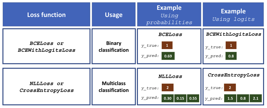
Please note that computing the cross-entropy loss by providing the logits, and not the class-membership probabilities, is usually preferred due to numerical stability reasons.

For binary classification, we can either provide logits as inputs to the loss function nn. BCEWithLogitsLoss ( ), or compute the probabilities based on the logits and feed them to the loss function nn.BCELoss ( ).
For multiclass classification, we can either provide logits as inputs to the loss function nn.CrossEntropyLoss( ), or compute the log probabilities based on the logits and feed them to the negative log-likelihood loss function nn.NLLLoss( ).

The following code will show you how to use these loss functions with two different formats, where either the logits or class-membership probabilities are given as inputs to the loss functions:

####### Binary Cross-entropy
logits = torch.tensor([0.8])
probas = torch.sigmoid(logits)
target = torch.tensor([1.0])

bce_loss_fn = nn.BCELoss()
bce_logits_loss_fn = nn.BCEWithLogitsLoss()

print(f'BCE (w Probas): {bce_loss_fn(probas, target):.4f}')
print(f'BCE (w Logits): {bce_logits_loss_fn(logits, target):.4f}')

 
####### Categorical Cross-entropy
logits = torch.tensor([[1.5, 0.8, 2.1]])
probas = torch.softmax(logits, dim=1)
target = torch.tensor([2])

cce_loss_fn = nn.NLLLoss()
cce_logits_loss_fn = nn.CrossEntropyLoss()

print(f'CCE (w Logits): {cce_logits_loss_fn(logits, target):.4f}')
print(f'CCE (w Probas): {cce_loss_fn(torch.log(probas), target):.4f}')

BCE (w Probas): 0.3711
BCE (w Logits): 0.3711
CCE (w Logits): 0.5996
CCE (w Probas): 0.5996

CNN with PyTorch¶

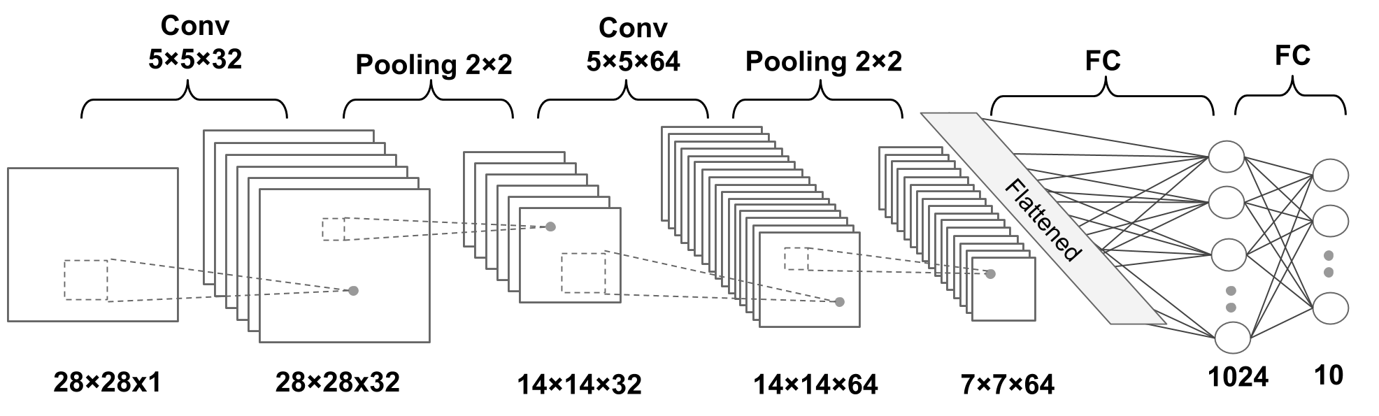
The dimensions of the tensors in each layer are as follows:

Input: $[batchsize \times 28 \times 28 \times 1]$
- 28×28 grayscale image × 1 channel
Conv_1: $[batchsize \times 28 \times 28 \times 32]$
- 5×5 kernel, using stride=1
- 32 output feature maps
Pooling_1: $[batchsize \times 14 \times 14 \times 32]$
- max-pooling operation, $P_{2 \times 2}$
- kernel_size=2 to shrink the size of the output feature maps
Conv_2: $[batchsize \times 14 \times 14 \times 64]$
- 5×5 kernel, using stride=1
- 64 output feature maps
Pooling_2: $[batchsize \times 7 \times 7 \times 64]$
- max-pooling operation, $P_{2 \times 2}$
- kernel_size=2 to shrink the size of the output feature maps
FC_1: $[batchsize \times 1024]$
FC_2 and softmax layer: $[batchsize×10]$

Loading and preprocessing the data¶

First, we will load the MNIST dataset using the torchvision module and construct the training and test sets. The MNIST dataset comes with a pre-specified training and test dataset partitioning scheme, but we also want to create a validation split from the train partition. Hence, we used the first 10,000 training examples for validation. Note that the images are not sorted by class label, so we do not have to worry about whether those validation set images are from the same classes.

import torchvision 
from torchvision import transforms 
image_path = './'
transform = transforms.Compose([transforms.ToTensor()])

mnist_dataset = torchvision.datasets.MNIST(root=image_path, 
                                           train=True, 
                                           transform=transform, 
                                           download=True)

from torch.utils.data import Subset
mnist_valid_dataset = Subset(mnist_dataset, torch.arange(10000)) 
mnist_train_dataset = Subset(mnist_dataset, torch.arange(10000, len(mnist_dataset)))
mnist_test_dataset = torchvision.datasets.MNIST(root=image_path, 
                                           train=False, 
                                           transform=transform, 
                                           download=False)

Downloading http://yann.lecun.com/exdb/mnist/train-images-idx3-ubyte.gz
Failed to download (trying next):
HTTP Error 404: Not Found

Downloading https://ossci-datasets.s3.amazonaws.com/mnist/train-images-idx3-ubyte.gz
Downloading https://ossci-datasets.s3.amazonaws.com/mnist/train-images-idx3-ubyte.gz to ./MNIST/raw/train-images-idx3-ubyte.gz

100%|██████████| 9912422/9912422 [00:00<00:00, 15888610.51it/s]

Extracting ./MNIST/raw/train-images-idx3-ubyte.gz to ./MNIST/raw

Downloading http://yann.lecun.com/exdb/mnist/train-labels-idx1-ubyte.gz
Failed to download (trying next):
HTTP Error 404: Not Found

Downloading https://ossci-datasets.s3.amazonaws.com/mnist/train-labels-idx1-ubyte.gz
Downloading https://ossci-datasets.s3.amazonaws.com/mnist/train-labels-idx1-ubyte.gz to ./MNIST/raw/train-labels-idx1-ubyte.gz

100%|██████████| 28881/28881 [00:00<00:00, 1007080.69it/s]

Extracting ./MNIST/raw/train-labels-idx1-ubyte.gz to ./MNIST/raw

Downloading http://yann.lecun.com/exdb/mnist/t10k-images-idx3-ubyte.gz

Failed to download (trying next):
HTTP Error 404: Not Found

Downloading https://ossci-datasets.s3.amazonaws.com/mnist/t10k-images-idx3-ubyte.gz
Downloading https://ossci-datasets.s3.amazonaws.com/mnist/t10k-images-idx3-ubyte.gz to ./MNIST/raw/t10k-images-idx3-ubyte.gz

100%|██████████| 1648877/1648877 [00:00<00:00, 8389081.16it/s]

Extracting ./MNIST/raw/t10k-images-idx3-ubyte.gz to ./MNIST/raw

Downloading http://yann.lecun.com/exdb/mnist/t10k-labels-idx1-ubyte.gz
Failed to download (trying next):
HTTP Error 404: Not Found

Downloading https://ossci-datasets.s3.amazonaws.com/mnist/t10k-labels-idx1-ubyte.gz
Downloading https://ossci-datasets.s3.amazonaws.com/mnist/t10k-labels-idx1-ubyte.gz to ./MNIST/raw/t10k-labels-idx1-ubyte.gz

100%|██████████| 4542/4542 [00:00<00:00, 4037839.93it/s]

Extracting ./MNIST/raw/t10k-labels-idx1-ubyte.gz to ./MNIST/raw

Next, we will construct the data loader with batches of 64 images for the training set and validation set, respectively. The labels are integers from 0 to 9, representing ten digits. Hence, we don’t need to do any scaling or further conversion.

from torch.utils.data import DataLoader


batch_size = 64
torch.manual_seed(1)
train_dl = DataLoader(mnist_train_dataset, batch_size, shuffle=True)
valid_dl = DataLoader(mnist_valid_dataset, batch_size, shuffle=False)

Implementing a CNN using the torch.nn module¶

It is worth mentioning that usually, when we read an image, the default dimension for the channels is the first dimension of the tensor array (or the second dimension considering the batch dimension). This is called the NCHW format, where

$N$ stands for the number of images within the batch,
$C$ stands for channels, and
$H$ and $W$ stand for height and width, respectively.

Cheatsheet¶
Conv2d: torch.nn.Conv2d
out_channels
kernel_size
stride
padding
MaxPool2d: torch.nn.MaxPool2d
kernel_size
stride
padding
Dropout torch.nn.Dropout
p

In the following code, we will use the Sequential class and add the convolution and pooling layers.

model = nn.Sequential()
model.add_module('conv1', nn.Conv2d(in_channels=1, out_channels=32, kernel_size=5, padding=2))
model.add_module('relu1', nn.ReLU())        
model.add_module('pool1', nn.MaxPool2d(kernel_size=2))   
model.add_module('conv2', nn.Conv2d(in_channels=32, out_channels=64, kernel_size=5, padding=2))
model.add_module('relu2', nn.ReLU())        
model.add_module('pool2', nn.MaxPool2d(kernel_size=2))

As discussed earlier, using same padding mode preserves the spatial dimensions (vertical and horizontal dimensions) of the feature maps such that the inputs and outputs have the same height and width (and the number of channels may only differ in terms of the number of filters used). As mentioned before, the spatial dimension of the output feature map is calculated by:

o=\left\lfloor\frac{n+2 p-m}{s}\right\rfloor+1

(1)

where $n$ is the spatial dimension of the input feature map, and $p, m$ , and $s$ denote the padding, kernel size, and stride, respectively. We obtain $p=2$ in order to achieve $o=i$ . The max-pooling layers with pooling size $2 \times 2$ and stride of 2 will reduce the spatial dimensions by half. (Note that if the stride parameter is not specified in MaxPool2D, by default, it is set equal to the pooling kernel size.)

By providing the input shape as a tuple $(4,1,28,28)(4$ images within the batch, 1 channel, and image size $28 \times 28)$ , specified in this example, we calculated the output to have a shape $(4,64,7,7)$ , indicating feature maps with 64 channels and a spatial size of $7 \times 7$ . The first dimension corresponds to the batch dimension, for which we used 4 arbitrarily.

# Compute the size of the feature map
x = torch.ones((4, 1, 28, 28))
model(x).shape

torch.Size([4, 64, 7, 7])

The next layer that we want to add is a fully connected layer for implementing a classifier on top of our convolutional and pooling layers. The input to this layer must have rank 2, that is, shape $[batchsize \times input\_units]$ . Thus, we need to flatten the output of the previous layers to meet this requirement for the fully connected layer:

model.add_module('flatten', nn.Flatten()) 

x = torch.ones((4, 1, 28, 28))
model(x).shape

torch.Size([4, 3136])

Next, we will add two fully connected layers with a dropout layer in between. The last fully connected layer, named ' fc2 ', has 10 output units for the 10 class labels in the MNIST dataset.

model.add_module('fc1', nn.Linear(3136, 1024)) 
model.add_module('relu3', nn.ReLU()) 
model.add_module('dropout', nn.Dropout(p=0.5)) 
model.add_module('fc2', nn.Linear(1024, 10))

device = torch.device("cuda:0")
# device = torch.device("cpu")

model = model.to(device)

In practice, we usually use the sofmax activation to obtain the class-membership probabilities of each input example, assuming that the classes are mutually exclusive, so the probabilities for each example sum to 1 . However, the softmax function is already used internally inside PyTorch’s CrossEntropyLoss implementation, which is why don’t have to explicitly add it as a layer after the output layer above. The following code will create the loss function and optimizer for the model.

loss_fn = nn.CrossEntropyLoss()
optimizer = torch.optim.Adam(model.parameters(), lr=0.001)

Now we can train the model by defining the following function. Note that using the designated settings for training model.train( ) and evaluation model.eval () will automatically set the mode for the dropout layer and rescale the hidden units appropriately so that we do not have to worry about that at all.

def train(model, num_epochs, train_dl, valid_dl):
    loss_hist_train = [0] * num_epochs
    accuracy_hist_train = [0] * num_epochs
    loss_hist_valid = [0] * num_epochs
    accuracy_hist_valid = [0] * num_epochs
    for epoch in range(num_epochs):
        model.train()
        for x_batch, y_batch in train_dl:
            x_batch = x_batch.to(device) 
            y_batch = y_batch.to(device) 
            pred = model(x_batch)
            loss = loss_fn(pred, y_batch)
            loss.backward()
            optimizer.step()
            optimizer.zero_grad()
            loss_hist_train[epoch] += loss.item()*y_batch.size(0)
            is_correct = (torch.argmax(pred, dim=1) == y_batch).float()
            accuracy_hist_train[epoch] += is_correct.sum().cpu()

        loss_hist_train[epoch] /= len(train_dl.dataset)
        accuracy_hist_train[epoch] /= len(train_dl.dataset)
        
        model.eval()
        with torch.no_grad():
            for x_batch, y_batch in valid_dl:
                x_batch = x_batch.to(device) 
                y_batch = y_batch.to(device) 
                pred = model(x_batch)
                loss = loss_fn(pred, y_batch)
                loss_hist_valid[epoch] += loss.item()*y_batch.size(0) 
                is_correct = (torch.argmax(pred, dim=1) == y_batch).float() 
                accuracy_hist_valid[epoch] += is_correct.sum().cpu()

        loss_hist_valid[epoch] /= len(valid_dl.dataset)
        accuracy_hist_valid[epoch] /= len(valid_dl.dataset)
        
        print(f'Epoch {epoch+1} accuracy: {accuracy_hist_train[epoch]:.4f} val_accuracy: {accuracy_hist_valid[epoch]:.4f}')
    return loss_hist_train, loss_hist_valid, accuracy_hist_train, accuracy_hist_valid

Next, we will train this CNN model and use the validation dataset that we created for monitoring the learning progress.

torch.manual_seed(1)
num_epochs = 20
hist = train(model, num_epochs, train_dl, valid_dl)

Epoch 1 accuracy: 0.9502 val_accuracy: 0.9824
Epoch 2 accuracy: 0.9843 val_accuracy: 0.9837
Epoch 3 accuracy: 0.9896 val_accuracy: 0.9839
Epoch 4 accuracy: 0.9916 val_accuracy: 0.9900
Epoch 5 accuracy: 0.9934 val_accuracy: 0.9901
Epoch 6 accuracy: 0.9947 val_accuracy: 0.9893
Epoch 7 accuracy: 0.9953 val_accuracy: 0.9897
Epoch 8 accuracy: 0.9961 val_accuracy: 0.9899
Epoch 9 accuracy: 0.9962 val_accuracy: 0.9915
Epoch 10 accuracy: 0.9967 val_accuracy: 0.9914
Epoch 11 accuracy: 0.9968 val_accuracy: 0.9893
Epoch 12 accuracy: 0.9971 val_accuracy: 0.9912
Epoch 13 accuracy: 0.9979 val_accuracy: 0.9912
Epoch 14 accuracy: 0.9979 val_accuracy: 0.9905
Epoch 15 accuracy: 0.9971 val_accuracy: 0.9913
Epoch 16 accuracy: 0.9983 val_accuracy: 0.9912
Epoch 17 accuracy: 0.9980 val_accuracy: 0.9896
Epoch 18 accuracy: 0.9978 val_accuracy: 0.9918
Epoch 19 accuracy: 0.9986 val_accuracy: 0.9908
Epoch 20 accuracy: 0.9981 val_accuracy: 0.9905

Once the 20 epochs of training are finished, we can visualize the learning curves.

import matplotlib.pyplot as plt


x_arr = np.arange(len(hist[0])) + 1

fig = plt.figure(figsize=(12, 4))
ax = fig.add_subplot(1, 2, 1)
ax.plot(x_arr, hist[0], '-o', label='Train loss')
ax.plot(x_arr, hist[1], '--<', label='Validation loss')
ax.set_xlabel('Epoch', size=15)
ax.set_ylabel('Loss', size=15)
ax.legend(fontsize=15)
ax = fig.add_subplot(1, 2, 2)
ax.plot(x_arr, hist[2], '-o', label='Train acc.')
ax.plot(x_arr, hist[3], '--<', label='Validation acc.')
ax.legend(fontsize=15)
ax.set_xlabel('Epoch', size=15)
ax.set_ylabel('Accuracy', size=15)

#plt.savefig('figures/14_13.png')
plt.show()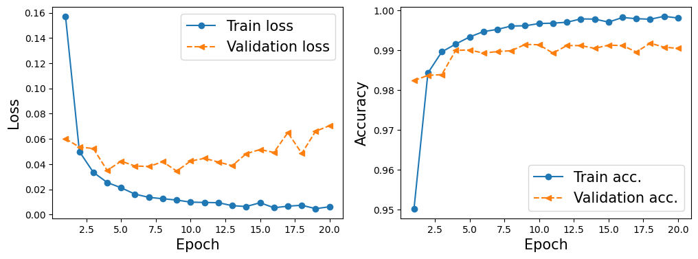

Now, we evaluate the trained model on the test dataset.

torch.cuda.synchronize()
model_cpu = model.cpu()
pred = model(mnist_test_dataset.data.unsqueeze(1) / 255.)
is_correct = (torch.argmax(pred, dim=1) == mnist_test_dataset.targets).float()
print(f'Test accuracy: {is_correct.mean():.4f}')

Test accuracy: 0.9922

Finally, we can get the prediction results in the form of class-membership probabilities and convert them to predicted labels by using the torch.argmax function to find the element with the maximum probability. We will do this for a batch of 12 examples and visualize the input and predicted labels.

fig = plt.figure(figsize=(12, 4))
for i in range(12):
    ax = fig.add_subplot(2, 6, i+1)
    ax.set_xticks([]); ax.set_yticks([])
    img = mnist_test_dataset[i][0][0, :, :]
    pred = model(img.unsqueeze(0).unsqueeze(1))
    y_pred = torch.argmax(pred)
    ax.imshow(img, cmap='gray_r')
    ax.text(0.9, 0.1, y_pred.item(), 
            size=15, color='blue',
            horizontalalignment='center',
            verticalalignment='center', 
            transform=ax.transAxes)
    
    
#plt.savefig('figures/14_14.png')
plt.show()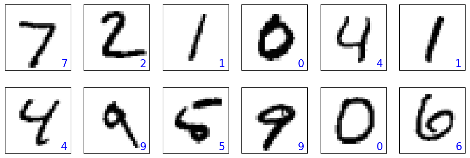

Save the trained model.

import os

if not os.path.exists('models'):
    os.mkdir('models')

path = 'models/mnist-cnn.ph'
torch.save(model, path)

Smile classification from face images using CNN¶

Loading the CelebA dataset¶

You can try setting download=True in the code cell below, however due to the daily download limits of the CelebA dataset, this will probably result in an error. Alternatively, we recommend trying the following:

You can download the files from the official CelebA website manually (https://mmlab.ie.cuhk.edu.hk/projects/CelebA.html)
or use our download link, https://drive.google.com/file/d/1m8-EBPgi5MRubrm6iQjafK2QMHDBMSfJ/view?usp=sharing (recommended).

If you use our download link, it will download a celeba.zip file,

which you need to unpack in the current directory where you are running the code.
In addition, please also make sure you unzip the img_align_celeba.zip file, which is inside the celeba folder.
Also, after downloading and unzipping the celeba folder, you need to run with the setting download=False instead of download=True (as shown in the code cell below).

In case you are encountering problems with this approach, please do not hesitate to open a new issue or start a discussion at https://github.com/rasbt/machine-learning-book so that we can provide you with additional information.

! pip install gdown
! mkdir ./celeba
! gdown --id 1m8-EBPgi5MRubrm6iQjafK2QMHDBMSfJ -O ./celeba/celeba.zip
! unzip ./celeba/celeba.zip -d ./celeba
! unzip ./celeba/celeba/img_align_celeba.zip -d ./celeba/celeba/

Looking in indexes: https://pypi.org/simple, https://pypi.ngc.nvidia.com
Requirement already satisfied: gdown in /usr/local/lib/python3.10/dist-packages (5.2.0)
Requirement already satisfied: beautifulsoup4 in /usr/local/lib/python3.10/dist-packages (from gdown) (4.12.2)
Requirement already satisfied: filelock in /usr/local/lib/python3.10/dist-packages (from gdown) (3.12.0)
Requirement already satisfied: requests[socks] in /usr/local/lib/python3.10/dist-packages (from gdown) (2.29.0)
Requirement already satisfied: tqdm in /usr/local/lib/python3.10/dist-packages (from gdown) (4.65.0)
Requirement already satisfied: soupsieve>1.2 in /usr/local/lib/python3.10/dist-packages (from beautifulsoup4->gdown) (2.4.1)
Requirement already satisfied: charset-normalizer<4,>=2 in /usr/local/lib/python3.10/dist-packages (from requests[socks]->gdown) (3.1.0)
Requirement already satisfied: certifi>=2017.4.17 in /usr/local/lib/python3.10/dist-packages (from requests[socks]->gdown) (2025.1.31)
Requirement already satisfied: urllib3<1.27,>=1.21.1 in /usr/local/lib/python3.10/dist-packages (from requests[socks]->gdown) (1.26.15)
Requirement already satisfied: idna<4,>=2.5 in /usr/local/lib/python3.10/dist-packages (from requests[socks]->gdown) (3.4)
Requirement already satisfied: PySocks!=1.5.7,>=1.5.6 in /usr/local/lib/python3.10/dist-packages (from requests[socks]->gdown) (1.7.1)
WARNING: Running pip as the 'root' user can result in broken permissions and conflicting behaviour with the system package manager. It is recommended to use a virtual environment instead: https://pip.pypa.io/warnings/venv
WARNING: You are using pip version 21.2.4; however, version 25.0.1 is available.
You should consider upgrading via the '/usr/bin/python -m pip install --upgrade pip' command.
/usr/local/lib/python3.10/dist-packages/gdown/__main__.py:140: FutureWarning: Option `--id` was deprecated in version 4.3.1 and will be removed in 5.0. You don't need to pass it anymore to use a file ID.
  warnings.warn(
Downloading...
From (original): https://drive.google.com/uc?id=1m8-EBPgi5MRubrm6iQjafK2QMHDBMSfJ
From (redirected): https://drive.google.com/uc?id=1m8-EBPgi5MRubrm6iQjafK2QMHDBMSfJ&confirm=t&uuid=a7c9b478-ff5e-47bf-a635-703cea0baa61
To: /home/vol-course/MyLectures/CNN/ch14/celeba/celeba.zip
100%|███████████████████████████████████████| 1.31G/1.31G [00:09<00:00, 137MB/s]
Archive:  ./celeba/celeba.zip
   creating: ./celeba/celeba/
  inflating: ./celeba/celeba/img_align_celeba.zip  
  inflating: ./celeba/__MACOSX/celeba/._img_align_celeba.zip  
  inflating: ./celeba/celeba/list_attr_celeba.txt  
  inflating: ./celeba/__MACOSX/celeba/._list_attr_celeba.txt  
  inflating: ./celeba/celeba/.DS_Store  
  inflating: ./celeba/__MACOSX/celeba/._.DS_Store  
  inflating: ./celeba/celeba/list_bbox_celeba.txt  
  inflating: ./celeba/__MACOSX/celeba/._list_bbox_celeba.txt  
  inflating: ./celeba/celeba/list_landmarks_align_celeba.txt  
  inflating: ./celeba/__MACOSX/celeba/._list_landmarks_align_celeba.txt  
  inflating: ./celeba/celeba/list_landmarks_celeba.txt  
  inflating: ./celeba/__MACOSX/celeba/._list_landmarks_celeba.txt  
  inflating: ./celeba/celeba/list_eval_partition.txt  
  inflating: ./celeba/__MACOSX/celeba/._list_eval_partition.txt  
  inflating: ./celeba/celeba/identity_CelebA.txt  
  inflating: ./celeba/__MACOSX/celeba/._identity_CelebA.txt

import torchvision

image_path = './celeba'  # Ensure the correct dataset directory
celeba_train_dataset = torchvision.datasets.CelebA(image_path, split='train', target_type='attr', download=False)
celeba_valid_dataset = torchvision.datasets.CelebA(image_path, split='valid', target_type='attr', download=False)
celeba_test_dataset = torchvision.datasets.CelebA(image_path, split='test', target_type='attr', download=False)

print('Train set:', len(celeba_train_dataset))
print('Validation set:', len(celeba_valid_dataset))
print('Test set:', len(celeba_test_dataset))

Train set: 162770
Validation set: 19867
Test set: 19962

Image transformation and data augmentation¶

Before training our CNN on the CelebA dataset for smile classification, we apply data augmentation techniques to enhance model robustness. This visualization showcases five common transformations, each demonstrated on a sample image:

Cropping to a Bounding Box – Extracts a region of interest to focus on the face.
Flipping (Horizontal Flip) – Introduces variation by mirroring the image, helping the model generalize better.
Adjusting Contrast – Enhances feature visibility by increasing contrast.
Adjusting Brightness – Simulates different lighting conditions.
Center Cropping & Resizing – Standardizes input size while preserving important facial features.

These augmentations help the CNN learn invariant features, improving performance on smile classification.

from torchvision import transforms 

## take 5 examples

fig = plt.figure(figsize=(16, 8.5))

## Column 1: cropping to a bounding-box
ax = fig.add_subplot(2, 5, 1)
img, attr = celeba_train_dataset[0]
ax.set_title('Crop to a \nbounding-box', size=15)
ax.imshow(img)
ax = fig.add_subplot(2, 5, 6)
img_cropped = transforms.functional.crop(img, 50, 20, 128, 128)
ax.imshow(img_cropped)

## Column 2: flipping (horizontally)
ax = fig.add_subplot(2, 5, 2)
img, attr = celeba_train_dataset[1]
ax.set_title('Flip (horizontal)', size=15)
ax.imshow(img)
ax = fig.add_subplot(2, 5, 7)
img_flipped = transforms.functional.hflip(img)
ax.imshow(img_flipped)

## Column 3: adjust contrast
ax = fig.add_subplot(2, 5, 3)
img, attr = celeba_train_dataset[2]
ax.set_title('Adjust constrast', size=15)
ax.imshow(img)
ax = fig.add_subplot(2, 5, 8)
img_adj_contrast = transforms.functional.adjust_contrast(img, contrast_factor=2)
ax.imshow(img_adj_contrast)

## Column 4: adjust brightness
ax = fig.add_subplot(2, 5, 4)
img, attr = celeba_train_dataset[3]
ax.set_title('Adjust brightness', size=15)
ax.imshow(img)
ax = fig.add_subplot(2, 5, 9)
img_adj_brightness = transforms.functional.adjust_brightness(img, brightness_factor=1.3)
ax.imshow(img_adj_brightness)

## Column 5: cropping from image center 
ax = fig.add_subplot(2, 5, 5)
img, attr = celeba_train_dataset[4]
ax.set_title('Center crop\nand resize', size=15)
ax.imshow(img)
ax = fig.add_subplot(2, 5, 10)
img_center_crop = transforms.functional.center_crop(img, [0.7*218, 0.7*178])
img_resized = transforms.functional.resize(img_center_crop, size=(218, 178))
ax.imshow(img_resized)
 
# plt.savefig('figures/14_14.png', dpi=300)
plt.show()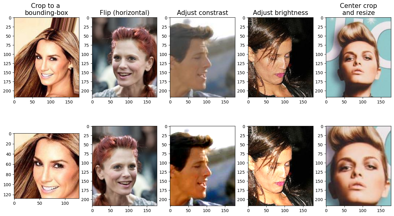

To improve our CNN’s ability to recognize smiles across diverse conditions, we apply a pipeline of augmentations in a stepwise manner. This visualization demonstrates how each transformation alters the original image:

Original Image – Raw input from the CelebA dataset.
Step 1: Random Crop – Extracts a random 178×178 region, ensuring the model learns from different facial regions.
Step 2: Random Horizontal Flip – Mirrors the image with a 50% probability, helping the model become invariant to orientation.
Step 3: Resize – Standardizes all images to 128×128 for consistent CNN input.

These augmentations help prevent overfitting and make the model more robust to real-world variations.

torch.manual_seed(1)

fig = plt.figure(figsize=(14, 12))

for i, (img, attr) in enumerate(celeba_train_dataset):
    ax = fig.add_subplot(3, 4, i*4+1)
    ax.imshow(img)
    if i == 0:
        ax.set_title('Orig.', size=15)
        
    ax = fig.add_subplot(3, 4, i*4+2)
    img_transform = transforms.Compose([transforms.RandomCrop([178, 178])])
    img_cropped = img_transform(img)
    ax.imshow(img_cropped)
    if i == 0:
        ax.set_title('Step 1: Random crop', size=15)

    ax = fig.add_subplot(3, 4, i*4+3)
    img_transform = transforms.Compose([transforms.RandomHorizontalFlip()])
    img_flip = img_transform(img_cropped)
    ax.imshow(img_flip)
    if i == 0:
        ax.set_title('Step 2: Random flip', size=15)

    ax = fig.add_subplot(3, 4, i*4+4)
    img_resized = transforms.functional.resize(img_flip, size=(128, 128))
    ax.imshow(img_resized)
    if i == 0:
        ax.set_title('Step 3: Resize', size=15)
    
    if i == 2:
        break
        
# plt.savefig('figures/14_15.png', dpi=300)
plt.show()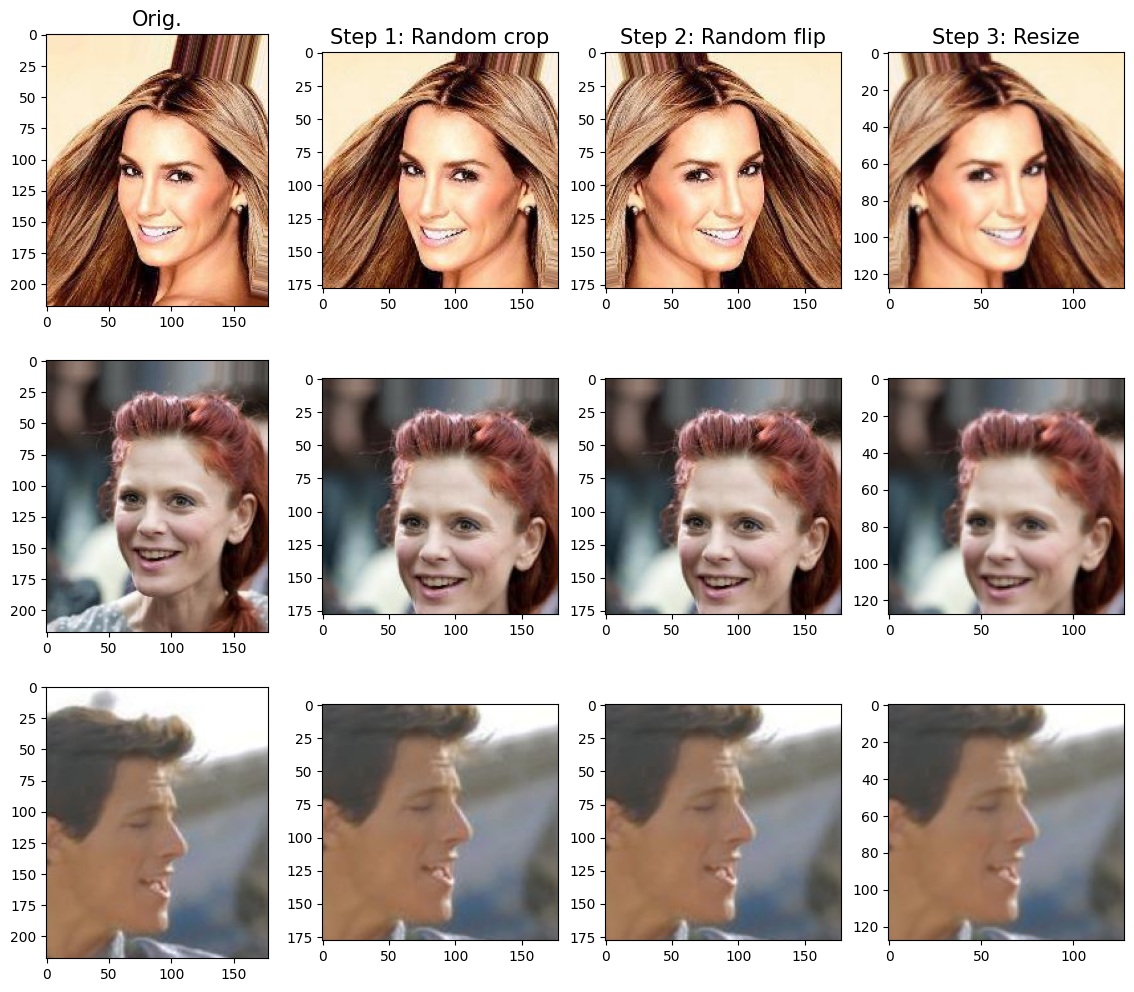

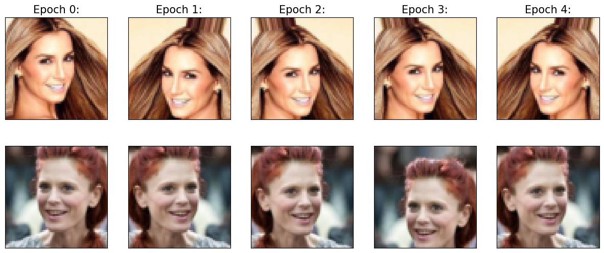
This code defines a data loading pipeline for training our CNN to classify smiles in the CelebA dataset. The key steps include:

Label Extraction – get_smile = lambda attr: attr[31] selects the attribute corresponding to smiling.
Training Data Augmentation:
- Random Crop (178×178): Crops a random region to introduce variation.
- Random Horizontal Flip: Simulates real-world variations in facial orientation.
- Resize to 64×64: Standardizes input size for CNN processing.
- ToTensor(): Converts images to PyTorch tensors.
DataLoader for Mini-batches – Loads images in batches of 2 for efficient training.
Visualization of Augmented Data Across Epochs –
- For each epoch, two images are sampled and displayed, illustrating how augmentation varies across training iterations.

This approach ensures that the CNN learns to recognize smiles robustly, despite variations in pose, cropping, and alignment.

get_smile = lambda attr: attr[31]
 
transform_train = transforms.Compose([
    transforms.RandomCrop([178, 178]),
    transforms.RandomHorizontalFlip(),
    transforms.Resize([64, 64]),
    transforms.ToTensor(),
])

transform = transforms.Compose([
    transforms.CenterCrop([178, 178]),
    transforms.Resize([64, 64]),
    transforms.ToTensor(),
])

from torch.utils.data import DataLoader

celeba_train_dataset = torchvision.datasets.CelebA(image_path, 
                                                   split='train', 
                                                   target_type='attr', 
                                                   download=False, 
                                                   transform=transform_train,
                                                   target_transform=get_smile)

torch.manual_seed(1)
data_loader = DataLoader(celeba_train_dataset, batch_size=2)

fig = plt.figure(figsize=(15, 6))

num_epochs = 5
for j in range(num_epochs):
    img_batch, label_batch = next(iter(data_loader))
    img = img_batch[0]
    ax = fig.add_subplot(2, 5, j + 1)
    ax.set_xticks([])
    ax.set_yticks([])
    ax.set_title(f'Epoch {j}:', size=15)
    ax.imshow(img.permute(1, 2, 0))

    img = img_batch[1]
    ax = fig.add_subplot(2, 5, j + 6)
    ax.set_xticks([])
    ax.set_yticks([])
    ax.imshow(img.permute(1, 2, 0))
      
    
#plt.savefig('figures/14_16.png', dpi=300)
plt.show()

Before training our CNN on the CelebA dataset, we define the training, validation, and test sets with the necessary transformations:

Dataset Splitting
- Training Set: 16,000 images (subset from the original train set).
- Validation Set: 1,000 images for model evaluation.
- Test Set: Full CelebA test set for final performance assessment.
Transformations for Consistency
- Training Transform (transform_train): Includes random cropping and horizontal flipping to introduce variation.
- Validation & Test Transform (transform): Uses center cropping to ensure consistency.
Data Loaders for Efficient Training
- Mini-batches (batch size = 32)
- Shuffling enabled for training, ensuring varied batches each epoch.
- No shuffling for validation and test, maintaining reproducibility.

celeba_valid_dataset = torchvision.datasets.CelebA(image_path, 
                                                   split='valid', 
                                                   target_type='attr', 
                                                   download=False, 
                                                   transform=transform,
                                                   target_transform=get_smile)

celeba_test_dataset = torchvision.datasets.CelebA(image_path, 
                                                   split='test', 
                                                   target_type='attr', 
                                                   download=False, 
                                                   transform=transform,
                                                   target_transform=get_smile)

from torch.utils.data import Subset
celeba_train_dataset = Subset(celeba_train_dataset, torch.arange(16000)) 
celeba_valid_dataset = Subset(celeba_valid_dataset, torch.arange(1000)) 
 
print('Train set:', len(celeba_train_dataset))
print('Validation set:', len(celeba_valid_dataset))

Train set: 16000
Validation set: 1000

batch_size = 32

torch.manual_seed(1)
train_dl = DataLoader(celeba_train_dataset, batch_size, shuffle=True)
valid_dl = DataLoader(celeba_valid_dataset, batch_size, shuffle=False)
test_dl = DataLoader(celeba_test_dataset, batch_size, shuffle=False)

Training a CNN Smile classifier¶

CNN Architecture Overview

Conv Layer 1:
- 3 input channels (RGB images) → 32 feature maps
- ReLU activation introduces non-linearity
- MaxPooling (2×2) reduces spatial dimensions
- Dropout (p=0.5) prevents overfitting
Conv Layer 2:
- 32 → 64 feature maps
- ReLU activation, MaxPooling (2×2), and Dropout (p=0.5)
Conv Layer 3:
- 64 → 128 feature maps
- ReLU activation and MaxPooling (2×2)
Conv Layer 4:
- 128 → 256 feature maps
- ReLU activation

This feature extraction process helps the CNN learn important spatial patterns in facial features related to smiling.

import torch.nn as nn

model = nn.Sequential()

model.add_module('conv1', nn.Conv2d(in_channels=3, out_channels=32, kernel_size=3, padding=1))
model.add_module('relu1', nn.ReLU())        
model.add_module('pool1', nn.MaxPool2d(kernel_size=2))  
model.add_module('dropout1', nn.Dropout(p=0.5)) 

model.add_module('conv2', nn.Conv2d(in_channels=32, out_channels=64, kernel_size=3, padding=1))
model.add_module('relu2', nn.ReLU())        
model.add_module('pool2', nn.MaxPool2d(kernel_size=2))   
model.add_module('dropout2', nn.Dropout(p=0.5)) 

model.add_module('conv3', nn.Conv2d(in_channels=64, out_channels=128, kernel_size=3, padding=1))
model.add_module('relu3', nn.ReLU())        
model.add_module('pool3', nn.MaxPool2d(kernel_size=2))   

model.add_module('conv4', nn.Conv2d(in_channels=128, out_channels=256, kernel_size=3, padding=1))
model.add_module('relu4', nn.ReLU())

After defining the convolutional layers, we finalize the model with pooling, flattening, and fully connected layers to map extracted features to a binary classification output (smiling or not smiling).

Final Model Updates:

Global Average Pooling
- AvgPool2d(kernel_size=8): Reduces the spatial dimensions, averaging feature maps from the last convolutional layer.
Flattening
- Flatten(): Converts the pooled feature maps into a 1D vector for the fully connected layer.
Fully Connected Layer
- Linear(256, 1): Maps the 256 features to a single output neuron.
- Sigmoid(): Ensures the output is between 0 and 1, representing the probability of a smile.

# example of a forward pass input, x (start)
x = torch.ones((4, 3, 64, 64))
model(x).shape

torch.Size([4, 256, 8, 8])

model.add_module('pool4', nn.AvgPool2d(kernel_size=8)) 
model.add_module('flatten', nn.Flatten()) 

x = torch.ones((4, 3, 64, 64))
model(x).shape

torch.Size([4, 256])

model.add_module('fc', nn.Linear(256, 1)) 
model.add_module('sigmoid', nn.Sigmoid())

# example of a forward pass input, x (end)
x = torch.ones((4, 3, 64, 64))
model(x).shape

torch.Size([4, 1])

model

Sequential(
  (conv1): Conv2d(3, 32, kernel_size=(3, 3), stride=(1, 1), padding=(1, 1))
  (relu1): ReLU()
  (pool1): MaxPool2d(kernel_size=2, stride=2, padding=0, dilation=1, ceil_mode=False)
  (dropout1): Dropout(p=0.5, inplace=False)
  (conv2): Conv2d(32, 64, kernel_size=(3, 3), stride=(1, 1), padding=(1, 1))
  (relu2): ReLU()
  (pool2): MaxPool2d(kernel_size=2, stride=2, padding=0, dilation=1, ceil_mode=False)
  (dropout2): Dropout(p=0.5, inplace=False)
  (conv3): Conv2d(64, 128, kernel_size=(3, 3), stride=(1, 1), padding=(1, 1))
  (relu3): ReLU()
  (pool3): MaxPool2d(kernel_size=2, stride=2, padding=0, dilation=1, ceil_mode=False)
  (conv4): Conv2d(128, 256, kernel_size=(3, 3), stride=(1, 1), padding=(1, 1))
  (relu4): ReLU()
  (pool4): AvgPool2d(kernel_size=8, stride=8, padding=0)
  (flatten): Flatten(start_dim=1, end_dim=-1)
  (fc): Linear(in_features=256, out_features=1, bias=True)
  (sigmoid): Sigmoid()
)

With our model architecture finalized, we now define the training process using Binary Cross-Entropy Loss (BCELoss) and Adam optimizer.

Key Training Steps:

Device Setup
- The model runs on GPU (cuda:0) if available for faster training.
- If needed, we can switch to CPU (device = torch.device("cpu")).
Loss Function & Optimizer
- BCELoss(): Measures how well the model predicts the probability of a smile.
- Adam() optimizer with a learning rate of 0.001 for adaptive learning.
Training Loop
- Forward Pass: Computes predictions and loss.
- Backward Pass: Updates model weights via gradient descent.
- Tracking Accuracy: Uses a threshold of 0.5 to determine smile classification.
Validation Loop
- After each epoch, the model is evaluated on the validation set without gradient computation (torch.no_grad()).
- Accuracy and loss are stored to monitor performance trends.

Training for 30 Epochs.

device = torch.device("cuda:0")
# device = torch.device("cpu")
model = model.to(device)

loss_fn = nn.BCELoss()
optimizer = torch.optim.Adam(model.parameters(), lr=0.001)

def train(model, num_epochs, train_dl, valid_dl):
    loss_hist_train = [0] * num_epochs
    accuracy_hist_train = [0] * num_epochs
    loss_hist_valid = [0] * num_epochs
    accuracy_hist_valid = [0] * num_epochs
    for epoch in range(num_epochs):
        model.train()
        for x_batch, y_batch in train_dl:
            x_batch = x_batch.to(device) 
            y_batch = y_batch.to(device) 
            pred = model(x_batch)[:, 0]
            loss = loss_fn(pred, y_batch.float())
            loss.backward()
            optimizer.step()
            optimizer.zero_grad()
            loss_hist_train[epoch] += loss.item()*y_batch.size(0)
            is_correct = ((pred>=0.5).float() == y_batch).float()
            accuracy_hist_train[epoch] += is_correct.sum().cpu()

        loss_hist_train[epoch] /= len(train_dl.dataset)
        accuracy_hist_train[epoch] /= len(train_dl.dataset)
        
        model.eval()
        with torch.no_grad():
            for x_batch, y_batch in valid_dl:
                x_batch = x_batch.to(device) 
                y_batch = y_batch.to(device) 
                pred = model(x_batch)[:, 0]
                loss = loss_fn(pred, y_batch.float())
                loss_hist_valid[epoch] += loss.item()*y_batch.size(0) 
                is_correct = ((pred>=0.5).float() == y_batch).float()
                accuracy_hist_valid[epoch] += is_correct.sum().cpu()

        loss_hist_valid[epoch] /= len(valid_dl.dataset)
        accuracy_hist_valid[epoch] /= len(valid_dl.dataset)
        
        print(f'Epoch {epoch+1} accuracy: {accuracy_hist_train[epoch]:.4f} val_accuracy: {accuracy_hist_valid[epoch]:.4f}')
    return loss_hist_train, loss_hist_valid, accuracy_hist_train, accuracy_hist_valid

torch.manual_seed(1)
num_epochs = 30
hist = train(model, num_epochs, train_dl, valid_dl)

Epoch 1 accuracy: 0.8598 val_accuracy: 0.8800
Epoch 2 accuracy: 0.8662 val_accuracy: 0.8880
Epoch 3 accuracy: 0.8651 val_accuracy: 0.8840
Epoch 4 accuracy: 0.8684 val_accuracy: 0.8900
Epoch 5 accuracy: 0.8712 val_accuracy: 0.8870
Epoch 6 accuracy: 0.8765 val_accuracy: 0.8910
Epoch 7 accuracy: 0.8770 val_accuracy: 0.8900
Epoch 8 accuracy: 0.8804 val_accuracy: 0.8970
Epoch 9 accuracy: 0.8813 val_accuracy: 0.8900
Epoch 10 accuracy: 0.8823 val_accuracy: 0.8930
Epoch 11 accuracy: 0.8826 val_accuracy: 0.8980
Epoch 12 accuracy: 0.8828 val_accuracy: 0.8930
Epoch 13 accuracy: 0.8844 val_accuracy: 0.8920
Epoch 14 accuracy: 0.8878 val_accuracy: 0.8970
Epoch 15 accuracy: 0.8884 val_accuracy: 0.8880
Epoch 16 accuracy: 0.8887 val_accuracy: 0.9020
Epoch 17 accuracy: 0.8907 val_accuracy: 0.8870
Epoch 18 accuracy: 0.8899 val_accuracy: 0.8970
Epoch 19 accuracy: 0.8981 val_accuracy: 0.9070
Epoch 20 accuracy: 0.8941 val_accuracy: 0.8970
Epoch 21 accuracy: 0.8957 val_accuracy: 0.9060
Epoch 22 accuracy: 0.8947 val_accuracy: 0.8990
Epoch 23 accuracy: 0.8925 val_accuracy: 0.8980
Epoch 24 accuracy: 0.8951 val_accuracy: 0.9100
Epoch 25 accuracy: 0.8932 val_accuracy: 0.9020
Epoch 26 accuracy: 0.8971 val_accuracy: 0.8950
Epoch 27 accuracy: 0.8954 val_accuracy: 0.9000
Epoch 28 accuracy: 0.8960 val_accuracy: 0.8920
Epoch 29 accuracy: 0.8994 val_accuracy: 0.9040
Epoch 30 accuracy: 0.8984 val_accuracy: 0.9060

To evaluate the model’s performance, we plot loss and accuracy trends over the 30 training epochs.

Plots Overview:

Left Plot: Loss vs. Epochs
- Shows how the training (Train loss) and validation (Validation loss) loss values decrease over time.
- A smooth decline indicates successful learning. If validation loss increases while training loss decreases, the model might be overfitting.
Right Plot: Accuracy vs. Epochs
- Displays training and validation accuracy trends.
- A steady increase in accuracy indicates improved classification performance.
- If the validation accuracy plateaus or decreases, it may signal overfitting or learning stagnation.

x_arr = np.arange(len(hist[0])) + 1

fig = plt.figure(figsize=(12, 4))
ax = fig.add_subplot(1, 2, 1)
ax.plot(x_arr, hist[0], '-o', label='Train loss')
ax.plot(x_arr, hist[1], '--<', label='Validation loss')
ax.legend(fontsize=15)
ax.set_xlabel('Epoch', size=15)
ax.set_ylabel('Loss', size=15)

ax = fig.add_subplot(1, 2, 2)
ax.plot(x_arr, hist[2], '-o', label='Train acc.')
ax.plot(x_arr, hist[3], '--<', label='Validation acc.')
ax.legend(fontsize=15)
ax.set_xlabel('Epoch', size=15)
ax.set_ylabel('Accuracy', size=15)

#plt.savefig('figures/14_17.png', dpi=300)
plt.show()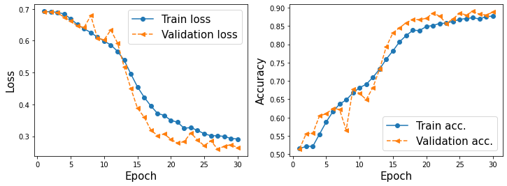

After training, we assess the final model performance on the unseen test set to measure generalization.

Key Steps in Testing:

Set the Model to Evaluation Mode
- model.eval() disables dropout and batch normalization updates.
- torch.no_grad() ensures no gradient computations, saving memory.
Batch-wise Predictions
- The model predicts smile probabilities (pred).
- A threshold of 0.5 determines smile classification (1 = smiling, 0 = not smiling).
- Predictions are compared to ground-truth labels.
Accuracy Calculation
- The total number of correct classifications is accumulated.
- The final accuracy is computed by dividing correct predictions by total test samples.

accuracy_test = 0

model.eval()
with torch.no_grad():
    for x_batch, y_batch in test_dl:
        x_batch = x_batch.to(device) 
        y_batch = y_batch.to(device) 
        pred = model(x_batch)[:, 0]
        is_correct = ((pred>=0.5).float() == y_batch).float()
        accuracy_test += is_correct.sum().cpu()
 
accuracy_test /= len(test_dl.dataset)
        
print(f'Test accuracy: {accuracy_test:.4f}')

Test accuracy: 0.9021

import os
if not os.path.exists('models'):
    os.mkdir('models')

path = 'models/celeba-cnn.ph'
torch.save(model, path)