

Predicting Continuous Target Variables with Regression Analysis
Package version checks
Add folder to path in order to load from the check_packages.py script:
import sys
sys.path.insert(0, '..')
Check recommended package versions:
# Install/verify packages needed for this notebook (Colab-safe)
import subprocess, sys

try:
    import mlxtend  # noqa: F401
except ImportError:
    subprocess.run([sys.executable, '-m', 'pip', 'install', '-q', 'mlxtend'], check=True)

import importlib

def check_packages(d):
    for pkg_name, min_version in d.items():
        try:
            imported = importlib.import_module(pkg_name)
            version = getattr(imported, '__version__', 'unknown')
            print(f'[OK] {pkg_name} {version}')
        except ImportError:
            print(f'[MISSING] {pkg_name} is not installed')

d = {
    'numpy': '1.21.2',
    'mlxtend': '0.19.0',
    'matplotlib': '3.4.3',
    'sklearn': '1.0',
    'pandas': '1.3.2',
}
check_packages(d)
[OK] numpy 2.0.2
[OK] mlxtend 0.23.4
[OK] matplotlib 3.10.0
[OK] sklearn 1.6.1
[OK] pandas 2.2.2
Chapter 09 - Predicting Continuous Target Variables with Regression Analysis
Overview
from IPython.display import Image
%matplotlib inline
Introducing linear regression
Simple linear regression
import os, urllib.request
os.makedirs('figures', exist_ok=True)
fig_path = 'figures/09_01.png'
if not os.path.exists(fig_path):
    url = 'https://raw.githubusercontent.com/rasbt/machine-learning-book/main/ch09/figures/09_01.png'
    try:
        urllib.request.urlretrieve(url, fig_path)
    except Exception as e:
        print(f'Could not download figure: {e}')
if os.path.exists(fig_path):
    display(Image(filename=fig_path, width=500))
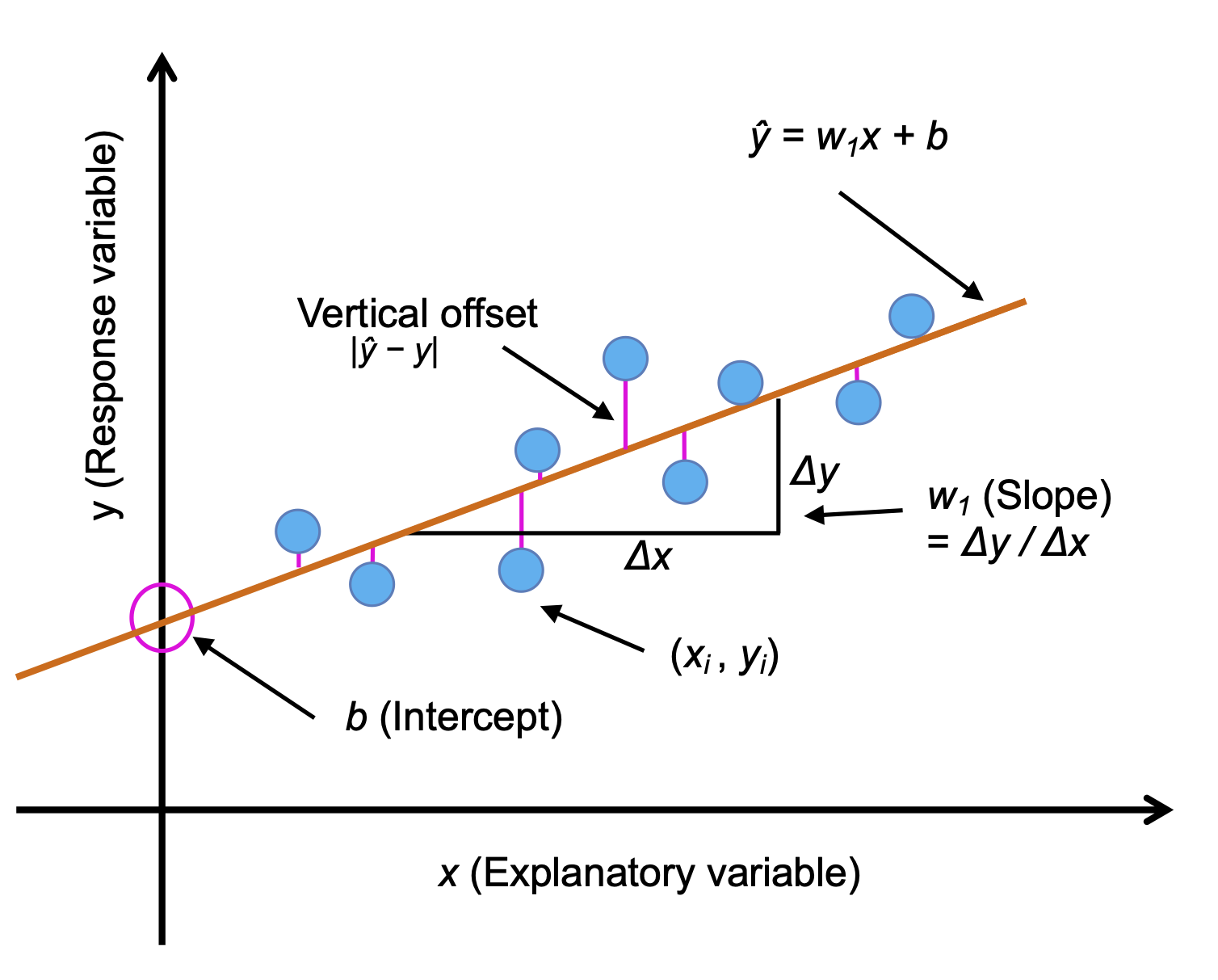
Multiple linear regression
import os, urllib.request
os.makedirs('figures', exist_ok=True)
fig_path = 'figures/09_01_2.png'
if not os.path.exists(fig_path):
    url = 'https://raw.githubusercontent.com/rasbt/machine-learning-book/main/ch09/figures/09_01_2.png'
    try:
        urllib.request.urlretrieve(url, fig_path)
    except Exception as e:
        print(f'Could not download figure: {e}')
if os.path.exists(fig_path):
    display(Image(filename=fig_path, width=500))
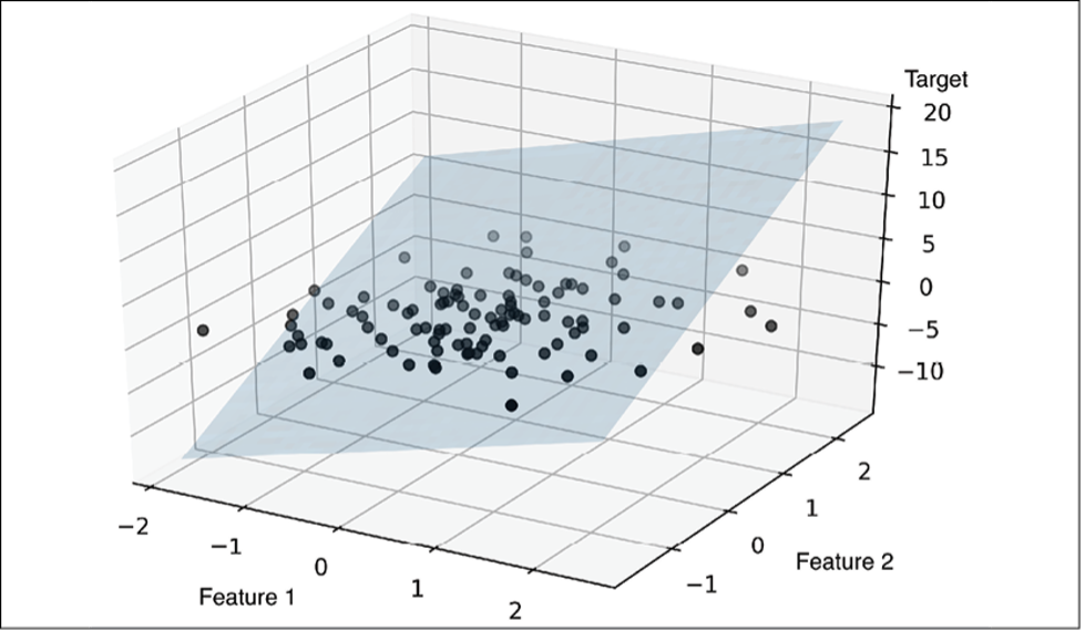
Exploring the Ames Housing dataset
Loading the Ames Housing dataset into a data frame
Dataset source: http://
jse .amstat .org /v19n3 /decock /AmesHousing .txt Dataset documentation: http://
jse .amstat .org /v19n3 /decock /DataDocumentation .txt Dataset write-up: http://
jse .amstat .org /v19n3 /decock .pdf
'Overall Qual': Rates the overall material and finish of the house10 Very Excellent 9 Excellent 8 Very Good 7 Good 6 Above Average 5 Average 4 Below Average 3 Fair 2 Poor 1 Very Poor'Overall Cond': Rates the overall condition of the house10 Very Excellent 9 Excellent 8 Very Good 7 Good 6 Above Average 5 Average 4 Below Average 3 Fair 2 Poor 1 Very Poor'Gr Liv Area': Above grade (ground) living area square feet'Central Air': Central air conditioningN No Y Yes'Total Bsmt SF': Total square feet of basement area'SalePrice': Sale price $$
import pandas as pd
from urllib.error import HTTPError, URLError

columns = ['Overall Qual', 'Overall Cond', 'Gr Liv Area',
           'Central Air', 'Total Bsmt SF', 'SalePrice']

try:
    df = pd.read_csv('http://jse.amstat.org/v19n3/decock/AmesHousing.txt',
                     sep='\t',
                     usecols=columns)
except (HTTPError, URLError, Exception) as e:
    # The JSE server can occasionally be unreachable / block automated requests.
    # Fall back to the book's GitHub-hosted copy of the same dataset.
    print('jse.amstat.org source failed ({}), falling back to GitHub copy.'.format(e))
    df = pd.read_csv(
        'https://raw.githubusercontent.com/rasbt/machine-learning-book/main/ch09/AmesHousing.txt',
        sep='\t',
        usecols=columns)

df.head()
Loading...
df.shape(2930, 6)df['Central Air'] = df['Central Air'].map({'N': 0, 'Y': 1})df.isnull().sum()Loading...
# remove rows that contain missing values

df = df.dropna(axis=0)
df.isnull().sum()
Loading...
Visualizing the important characteristics of a dataset
import matplotlib.pyplot as plt
from mlxtend.plotting import scatterplotmatrix
scatterplotmatrix(df.values, figsize=(12, 10),
names=df.columns, alpha=0.5)
plt.tight_layout()
#plt.savefig('figures/09_04.png', dpi=300)
plt.show()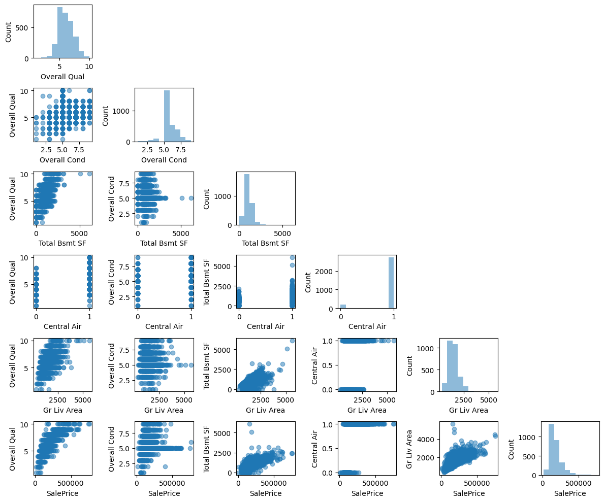
import numpy as np
from mlxtend.plotting import heatmap


cm = np.corrcoef(df.values.T)
hm = heatmap(cm, row_names=df.columns, column_names=df.columns)

plt.tight_layout()
#plt.savefig('figures/09_05.png', dpi=300)
plt.show()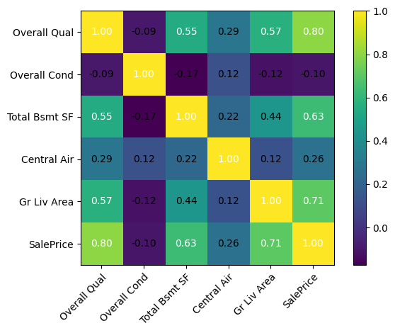
Implementing an ordinary least squares linear regression model
...
Solving regression for regression parameters with gradient descent
class LinearRegressionGD:
    def __init__(self, eta=0.01, n_iter=50, random_state=1):
        self.eta = eta
        self.n_iter = n_iter
        self.random_state = random_state

    def fit(self, X, y):
        rgen = np.random.RandomState(self.random_state)
        self.w_ = rgen.normal(loc=0.0, scale=0.01, size=X.shape[1])
        self.b_ = np.array([0.])
        self.losses_ = []

        for i in range(self.n_iter):
            output = self.net_input(X)
            errors = (y - output)
            self.w_ += self.eta * 2.0 * X.T.dot(errors) / X.shape[0]
            self.b_ += self.eta * 2.0 * errors.mean()
            loss = (errors**2).mean()
            self.losses_.append(loss)
        return self

    def net_input(self, X):
        return np.dot(X, self.w_) + self.b_

    def predict(self, X):
        return self.net_input(X)
X = df[['Gr Liv Area']].values
y = df['SalePrice'].valuesfrom sklearn.preprocessing import StandardScaler
sc_x = StandardScaler()
sc_y = StandardScaler()
X_std = sc_x.fit_transform(X)
y_std = sc_y.fit_transform(y[:, np.newaxis]).flatten()lr = LinearRegressionGD(eta=0.1)
lr.fit(X_std, y_std)<__main__.LinearRegressionGD at 0x79aae40a8830>plt.plot(range(1, lr.n_iter+1), lr.losses_)
plt.ylabel('MSE')
plt.xlabel('Epoch')
plt.tight_layout()
#plt.savefig('figures/09_06.png', dpi=300)
plt.show()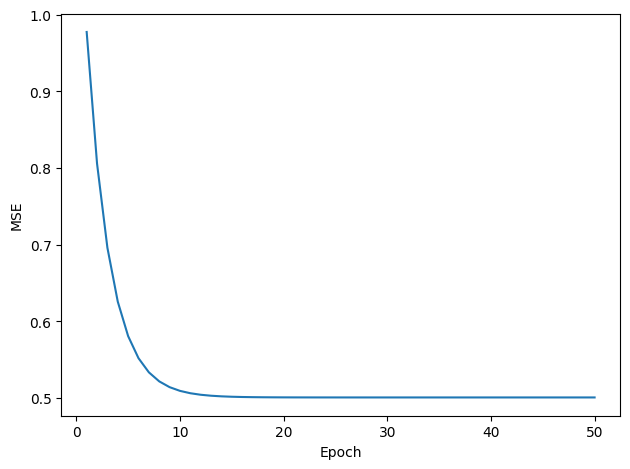
def lin_regplot(X, y, model):
plt.scatter(X, y, c='steelblue', edgecolor='white', s=70)
plt.plot(X, model.predict(X), color='black', lw=2)
returnlin_regplot(X_std, y_std, lr)
plt.xlabel('Living area above ground (standardized)')
plt.ylabel('Sale price (standardized)')
#plt.savefig('figures/09_07.png', dpi=300)
plt.show()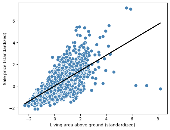
feature_std = sc_x.transform(np.array([[2500]]))
target_std = lr.predict(feature_std)
target_reverted = sc_y.inverse_transform(target_std.reshape(-1, 1))
print(f'Sale price: ${target_reverted.flatten()[0]:.2f}')Sale price: $292507.07
print(f'Slope: {lr.w_[0]:.3f}')
print(f'Intercept: {lr.b_[0]:.3f}')Slope: 0.707
Intercept: -0.000
Estimating the coefficient of a regression model via scikit-learn
from sklearn.linear_model import LinearRegressionslr = LinearRegression()
slr.fit(X, y)
y_pred = slr.predict(X)
print(f'Slope: {slr.coef_[0]:.3f}')
print(f'Intercept: {slr.intercept_:.3f}')Slope: 111.666
Intercept: 13342.979
lin_regplot(X, y, slr)
plt.xlabel('Living area above ground in square feet')
plt.ylabel('Sale price in U.S. dollars')
plt.tight_layout()
#plt.savefig('figures/09_08.png', dpi=300)
plt.show()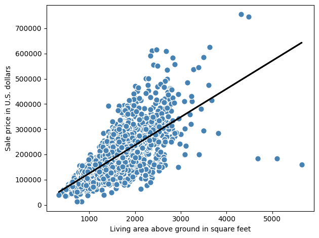
Normal Equations alternative:
# adding a column vector of "ones"
Xb = np.hstack((np.ones((X.shape[0], 1)), X))
w = np.zeros(X.shape[1])
z = np.linalg.inv(np.dot(Xb.T, Xb))
w = np.dot(z, np.dot(Xb.T, y))
print(f'Slope: {w[1]:.3f}')
print(f'Intercept: {w[0]:.3f}')Slope: 111.666
Intercept: 13342.979
Fitting a robust regression model using RANSAC
from sklearn.linear_model import RANSACRegressor
ransac = RANSACRegressor(LinearRegression(),
max_trials=100, # default
min_samples=0.95,
loss='absolute_error', # default
residual_threshold=None, # default
random_state=123)
ransac.fit(X, y)
inlier_mask = ransac.inlier_mask_
outlier_mask = np.logical_not(inlier_mask)
line_X = np.arange(3, 10, 1)
line_y_ransac = ransac.predict(line_X[:, np.newaxis])
plt.scatter(X[inlier_mask], y[inlier_mask],
c='steelblue', edgecolor='white',
marker='o', label='Inliers')
plt.scatter(X[outlier_mask], y[outlier_mask],
c='limegreen', edgecolor='white',
marker='s', label='Outliers')
plt.plot(line_X, line_y_ransac, color='black', lw=2)
plt.xlabel('Living area above ground in square feet')
plt.ylabel('Sale price in U.S. dollars')
plt.legend(loc='upper left')
plt.tight_layout()
#plt.savefig('figures/09_09.png', dpi=300)
plt.show()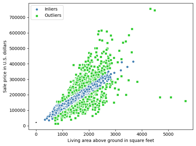
print(f'Slope: {ransac.estimator_.coef_[0]:.3f}')
print(f'Intercept: {ransac.estimator_.intercept_:.3f}')Slope: 106.348
Intercept: 20190.093
def median_absolute_deviation(data):
return np.median(np.abs(data - np.median(data)))
median_absolute_deviation(y)np.float64(37000.0)ransac = RANSACRegressor(LinearRegression(),
max_trials=100, # default
min_samples=0.95,
loss='absolute_error', # default
residual_threshold=65000, # default
random_state=123)
ransac.fit(X, y)
inlier_mask = ransac.inlier_mask_
outlier_mask = np.logical_not(inlier_mask)
line_X = np.arange(3, 10, 1)
line_y_ransac = ransac.predict(line_X[:, np.newaxis])
plt.scatter(X[inlier_mask], y[inlier_mask],
c='steelblue', edgecolor='white',
marker='o', label='Inliers')
plt.scatter(X[outlier_mask], y[outlier_mask],
c='limegreen', edgecolor='white',
marker='s', label='Outliers')
plt.plot(line_X, line_y_ransac, color='black', lw=2)
plt.xlabel('Living area above ground in square feet')
plt.ylabel('Sale price in U.S. dollars')
plt.legend(loc='upper left')
plt.tight_layout()
#plt.savefig('figures/09_10.png', dpi=300)
plt.show()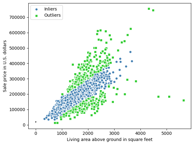
print(f'Slope: {ransac.estimator_.coef_[0]:.3f}')
print(f'Intercept: {ransac.estimator_.intercept_:.3f}')Slope: 105.631
Intercept: 18314.587
Evaluating the performance of linear regression models
from sklearn.model_selection import train_test_split
target = 'SalePrice'
features = df.columns[df.columns != target]
X = df[features].values
y = df[target].values
X_train, X_test, y_train, y_test = train_test_split(
X, y, test_size=0.3, random_state=123)slr = LinearRegression()
slr.fit(X_train, y_train)
y_train_pred = slr.predict(X_train)
y_test_pred = slr.predict(X_test)x_max = np.max([np.max(y_train_pred), np.max(y_test_pred)])
x_min = np.min([np.min(y_train_pred), np.min(y_test_pred)])
fig, (ax1, ax2) = plt.subplots(1, 2, figsize=(7, 3), sharey=True)
ax1.scatter(y_test_pred, y_test_pred - y_test,
c='limegreen', marker='s', edgecolor='white',
label='Test data')
ax2.scatter(y_train_pred, y_train_pred - y_train,
c='steelblue', marker='o', edgecolor='white',
label='Training data')
ax1.set_ylabel('Residuals')
for ax in (ax1, ax2):
ax.set_xlabel('Predicted values')
ax.legend(loc='upper left')
ax.hlines(y=0, xmin=x_min-100, xmax=x_max+100, color='black', lw=2)
plt.tight_layout()
#plt.savefig('figures/09_11.png', dpi=300)
plt.show()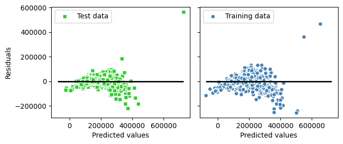
from sklearn.metrics import mean_squared_error
mse_train = mean_squared_error(y_train, y_train_pred)
mse_test = mean_squared_error(y_test, y_test_pred)
print(f'MSE train: {mse_train:.2f}')
print(f'MSE test: {mse_test:.2f}')MSE train: 1497216245.85
MSE test: 1516565821.00
from sklearn.metrics import mean_absolute_error
mae_train = mean_absolute_error(y_train, y_train_pred)
mae_test = mean_absolute_error(y_test, y_test_pred)
print(f'MAE train: {mae_train:.2f}')
print(f'MAE test: {mae_test:.2f}')MAE train: 25983.03
MAE test: 24921.29
from sklearn.metrics import r2_score
r2_train = r2_score(y_train, y_train_pred)
r2_test =r2_score(y_test, y_test_pred)
print(f'R^2 train: {r2_train:.2f}')
print(f'R^2 test: {r2_test:.2f}')R^2 train: 0.77
R^2 test: 0.75
Using regularized methods for regression
from sklearn.linear_model import Lasso
lasso = Lasso(alpha=1.0)
lasso.fit(X_train, y_train)
y_train_pred = lasso.predict(X_train)
y_test_pred = lasso.predict(X_test)
print(lasso.coef_)[26251.38276394 804.70816337 41.94651964 11364.80761309
55.67855548]
train_mse = mean_squared_error(y_train, y_train_pred)
test_mse = mean_squared_error(y_test, y_test_pred)
print(f'MSE train: {train_mse:.3f}, test: {test_mse:.3f}')
train_r2 = r2_score(y_train, y_train_pred)
test_r2 = r2_score(y_test, y_test_pred)
print(f'R^2 train: {train_r2:.3f}, {test_r2:.3f}')MSE train: 1497216262.014, test: 1516576825.348
R^2 train: 0.769, 0.752
Ridge regression:
from sklearn.linear_model import Ridge
ridge = Ridge(alpha=1.0)LASSO regression:
from sklearn.linear_model import Lasso
lasso = Lasso(alpha=1.0)Elastic Net regression:
from sklearn.linear_model import ElasticNet
elanet = ElasticNet(alpha=1.0, l1_ratio=0.5)Turning a linear regression model into a curve - polynomial regression
X = np.array([258.0, 270.0, 294.0,
320.0, 342.0, 368.0,
396.0, 446.0, 480.0, 586.0])\
[:, np.newaxis]
y = np.array([236.4, 234.4, 252.8,
298.6, 314.2, 342.2,
360.8, 368.0, 391.2,
390.8])from sklearn.preprocessing import PolynomialFeatures
lr = LinearRegression()
pr = LinearRegression()
quadratic = PolynomialFeatures(degree=2)
X_quad = quadratic.fit_transform(X)# fit linear features
lr.fit(X, y)
X_fit = np.arange(250, 600, 10)[:, np.newaxis]
y_lin_fit = lr.predict(X_fit)
# fit quadratic features
pr.fit(X_quad, y)
y_quad_fit = pr.predict(quadratic.fit_transform(X_fit))
# plot results
plt.scatter(X, y, label='Training points')
plt.plot(X_fit, y_lin_fit, label='Linear fit', linestyle='--')
plt.plot(X_fit, y_quad_fit, label='Quadratic fit')
plt.xlabel('Explanatory variable')
plt.ylabel('Predicted or known target values')
plt.legend(loc='upper left')
plt.tight_layout()
#plt.savefig('figures/09_12.png', dpi=300)
plt.show()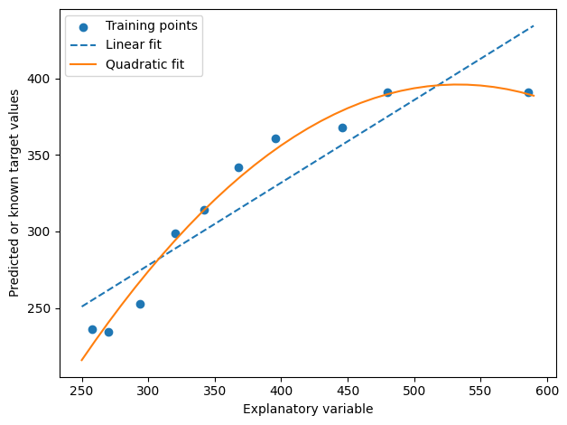
y_lin_pred = lr.predict(X)
y_quad_pred = pr.predict(X_quad)mse_lin = mean_squared_error(y, y_lin_pred)
mse_quad = mean_squared_error(y, y_quad_pred)
print(f'Training MSE linear: {mse_lin:.3f}'
f', quadratic: {mse_quad:.3f}')
r2_lin = r2_score(y, y_lin_pred)
r2_quad = r2_score(y, y_quad_pred)
print(f'Training R^2 linear: {r2_lin:.3f}'
f', quadratic: {r2_quad:.3f}')Training MSE linear: 569.780, quadratic: 61.330
Training R^2 linear: 0.832, quadratic: 0.982
Modeling nonlinear relationships in the Ames Housing dataset
import os
os.makedirs('figures', exist_ok=True)
X = df[['Gr Liv Area']].values
y = df['SalePrice'].values
X = X[(df['Gr Liv Area'] < 4000)]
y = y[(df['Gr Liv Area'] < 4000)]
regr = LinearRegression()
# create quadratic features
quadratic = PolynomialFeatures(degree=2)
cubic = PolynomialFeatures(degree=3)
X_quad = quadratic.fit_transform(X)
X_cubic = cubic.fit_transform(X)
# fit features
X_fit = np.arange(X.min()-1, X.max()+2, 1)[:, np.newaxis]
regr = regr.fit(X, y)
y_lin_fit = regr.predict(X_fit)
linear_r2 = r2_score(y, regr.predict(X))
regr = regr.fit(X_quad, y)
y_quad_fit = regr.predict(quadratic.fit_transform(X_fit))
quadratic_r2 = r2_score(y, regr.predict(X_quad))
regr = regr.fit(X_cubic, y)
y_cubic_fit = regr.predict(cubic.fit_transform(X_fit))
cubic_r2 = r2_score(y, regr.predict(X_cubic))
# plot results
plt.scatter(X, y, label='Training points', color='lightgray')
plt.plot(X_fit, y_lin_fit,
label=f'Linear (d=1), $R^2$={linear_r2:.2f}',
color='blue',
lw=2,
linestyle=':')
plt.plot(X_fit, y_quad_fit,
label=f'Quadratic (d=2), $R^2$={quadratic_r2:.2f}',
color='red',
lw=2,
linestyle='-')
plt.plot(X_fit, y_cubic_fit,
label=f'Cubic (d=3), $R^2$={cubic_r2:.2f}',
color='green',
lw=2,
linestyle='--')
plt.xlabel('Living area above ground in square feet')
plt.ylabel('Sale price in U.S. dollars')
plt.legend(loc='upper left')
plt.tight_layout()
plt.savefig('figures/09_13.png', dpi=300)
plt.show()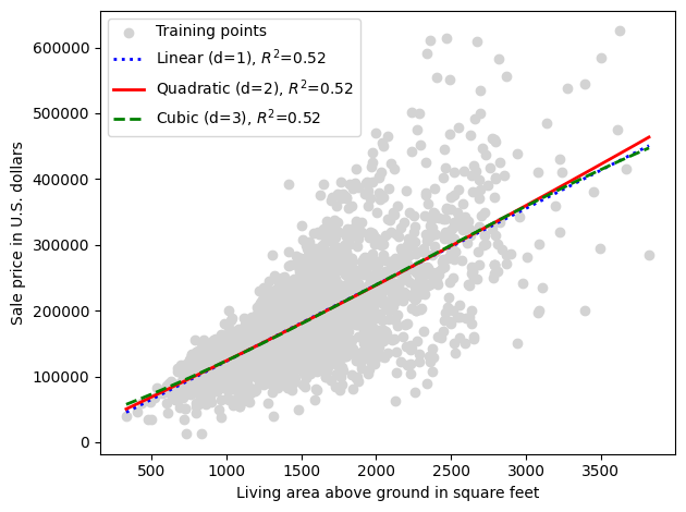
X = df[['Overall Qual']].values
y = df['SalePrice'].values


regr = LinearRegression()

# create quadratic features
quadratic = PolynomialFeatures(degree=2)
cubic = PolynomialFeatures(degree=3)
X_quad = quadratic.fit_transform(X)
X_cubic = cubic.fit_transform(X)

# fit features
X_fit = np.arange(X.min()-1, X.max()+2, 1)[:, np.newaxis]

regr = regr.fit(X, y)
y_lin_fit = regr.predict(X_fit)
linear_r2 = r2_score(y, regr.predict(X))

regr = regr.fit(X_quad, y)
y_quad_fit = regr.predict(quadratic.fit_transform(X_fit))
quadratic_r2 = r2_score(y, regr.predict(X_quad))

regr = regr.fit(X_cubic, y)
y_cubic_fit = regr.predict(cubic.fit_transform(X_fit))
cubic_r2 = r2_score(y, regr.predict(X_cubic))


# plot results
plt.scatter(X, y, label='Training points', color='lightgray')

plt.plot(X_fit, y_lin_fit,
         label=f'Linear (d=1), $R^2$={linear_r2:.2f}',
         color='blue',
         lw=2,
         linestyle=':')

plt.plot(X_fit, y_quad_fit,
         label=f'Quadratic (d=2), $R^2$={quadratic_r2:.2f}',
         color='red',
         lw=2,
         linestyle='-')

plt.plot(X_fit, y_cubic_fit,
         label=f'Cubic (d=3), $R^2$={cubic_r2:.2f}',
         color='green',
         lw=2,
         linestyle='--')


plt.xlabel('Overall quality of the house')
plt.ylabel('Sale price in U.S. dollars')
plt.legend(loc='upper left')

plt.tight_layout()
#plt.savefig('figures/09_14.png', dpi=300)
plt.show()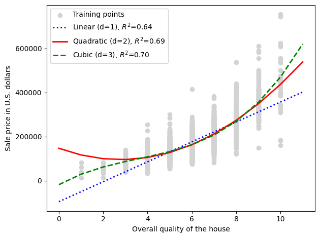
Dealing with nonlinear relationships using random forests
...
Decision tree regression
from sklearn.tree import DecisionTreeRegressor


X = df[['Gr Liv Area']].values
y = df['SalePrice'].values


tree = DecisionTreeRegressor(max_depth=3)
tree.fit(X, y)
sort_idx = X.flatten().argsort()

lin_regplot(X[sort_idx], y[sort_idx], tree)
plt.xlabel('Living area above ground in square feet')
plt.ylabel('Sale price in U.S. dollars')

plt.tight_layout()
#plt.savefig('figures/09_15.png', dpi=300)
plt.show()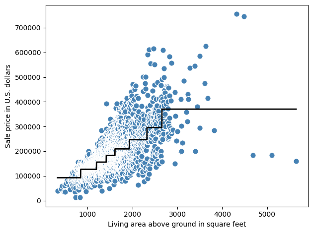
tree_r2 = r2_score(y, tree.predict(X))
tree_r20.5144569334885711Random forest regression
target = 'SalePrice'
features = df.columns[df.columns != target]

X = df[features].values
y = df[target].values

X_train, X_test, y_train, y_test = train_test_split(
    X, y, test_size=0.3, random_state=123)
from sklearn.ensemble import RandomForestRegressor
forest = RandomForestRegressor(n_estimators=1000,
criterion='squared_error',
random_state=1,
n_jobs=-1)
forest.fit(X_train, y_train)
y_train_pred = forest.predict(X_train)
y_test_pred = forest.predict(X_test)
mae_train = mean_absolute_error(y_train, y_train_pred)
mae_test = mean_absolute_error(y_test, y_test_pred)
print(f'MAE train: {mae_train:.2f}')
print(f'MAE test: {mae_test:.2f}')
r2_train = r2_score(y_train, y_train_pred)
r2_test =r2_score(y_test, y_test_pred)
print(f'R^2 train: {r2_train:.2f}')
print(f'R^2 test: {r2_test:.2f}')MAE train: 8305.18
MAE test: 20821.77
R^2 train: 0.98
R^2 test: 0.85
x_max = np.max([np.max(y_train_pred), np.max(y_test_pred)])
x_min = np.min([np.min(y_train_pred), np.min(y_test_pred)])

fig, (ax1, ax2) = plt.subplots(1, 2, figsize=(7, 3), sharey=True)

ax1.scatter(y_test_pred, y_test_pred - y_test,
            c='limegreen', marker='s', edgecolor='white',
            label='Test data')
ax2.scatter(y_train_pred, y_train_pred - y_train,
            c='steelblue', marker='o', edgecolor='white',
            label='Training data')
ax1.set_ylabel('Residuals')

for ax in (ax1, ax2):
    ax.set_xlabel('Predicted values')
    ax.legend(loc='upper left')
    ax.hlines(y=0, xmin=x_min-100, xmax=x_max+100, color='black', lw=2)

plt.tight_layout()

#plt.savefig('figures/09_16.png', dpi=300)
plt.show()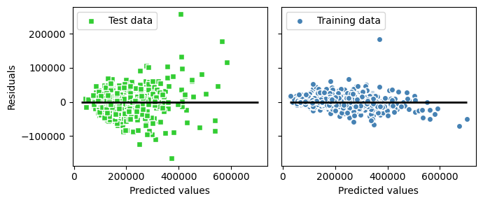
Summary
...
Readers may ignore the next cell.
# Optional utility script from the book's own repo (not included here) that
# converts this notebook to a .py file. Skipped safely when not present.
import os
script = '../.convert_notebook_to_script.py'
if os.path.exists(script):
    get_ipython().system('python {script} --input ch09-BAJ.ipynb --output ch09-BAJ.py')
else:
    print('Skipping: convert_notebook_to_script.py not present in this environment.')
Skipping: convert_notebook_to_script.py not present in this environment.