Building Good Training Datasets — Data Preprocessing¶

Package version checks¶

Add folder to path in order to load from the check_packages.py script:

Check recommended package versions:

Chapter 4 - Building Good Training Datasets – Data Preprocessing¶

Overview¶

• Dealing with missing data

  • Identifying missing values in tabular data

  • Eliminating training examples or features with missing values

  • Imputing missing values

  • Understanding the scikit-learn estimator API

• Handling categorical data

  • Nominal and ordinal features

  • Mapping ordinal features

  • Encoding class labels

  • Performing one-hot encoding on nominal features

• Partitioning a dataset into a separate training and test set

• Bringing features onto the same scale

• Selecting meaningful features

  • L1 and L2 regularization as penalties against model complexity

  • A geometric interpretation of L2 regularization

  • Sparse solutions with L1 regularization

  • Sequential feature selection algorithms

• Assessing feature importance with Random Forests

• Summary

Dealing with missing data¶

Identifying missing values in tabular data¶

This code is using the Pandas library to read a CSV data file from a string. The string is defined as csv_data, which contains a 4-column data table.

The code then checks the version of Python being used and converts the string to unicode if the version is 2.7 or earlier.

Finally, the code creates a Pandas DataFrame df by using the pd.read_csv function and passing in the string data using the StringIO function from the io library. The resulting DataFrame df contains the data from the CSV string.

The second code block uses the isnull() method from the pandas library to check for missing values in the dataframe df. The sum() method is then applied on the resulting boolean dataframe to count the number of missing values in each column. The result is a pandas series that displays the count of missing values in each column.

The code df.values accesses the underlying NumPy array of the Pandas DataFrame df. The values attribute returns a NumPy array representation of the DataFrame, allowing for easy integration with other numerical libraries in Python. This can be useful for performing numerical operations or passing the data to a machine learning model.

Eliminating training examples or features with missing values¶

The code is removing rows that contain missing values from the dataframe “df”. The “dropna” method is used to drop missing values in the dataframe. The “axis” parameter is set to 0, which indicates that we want to drop the rows that contain missing values. The resulting dataframe will only contain rows with no missing values.

The code df.dropna(how='all') will drop only the rows where all columns contain NaN values. In this case, if a row has at least one non-NaN value, it will be kept and not dropped. This is useful when you want to remove only the rows that have no information at all, and keep the ones that contain at least some data.

The code df.dropna(thresh=4) will drop rows in the pandas DataFrame df that have less than 4 non-null values. The argument thresh specifies the minimum number of non-null values a row must have in order to be kept. In this case, thresh=4 means that only rows with 4 or more non-null values will be kept, and any row with less than 4 non-null values will be dropped.

Imputing missing values¶

Impute Missing Values via the Column Mean¶

The code below uses the SimpleImputer class from scikit-learn’s impute module to fill in missing values in a pandas DataFrame df with the mean value of each column. The missing values are represented by np.nan.

from sklearn.impute import SimpleImputer
import numpy as np

# Create an instance of the SimpleImputer class
imr = SimpleImputer(missing_values=np.nan, strategy='mean')

# Fit the imputer to the data
imr = imr.fit(df.values)

# Transform the data to fill in the missing values
imputed_data = imr.transform(df.values)

# Preview the imputed data
print(imputed_data)

The code df.fillna(df.mean()) replaces the missing values in the pandas dataframe df with the mean value of each column.

This code first computes the mean of each column by calling df.mean(). The resulting Series is then passed to the fillna method, which replaces the missing values in df with the corresponding mean values.

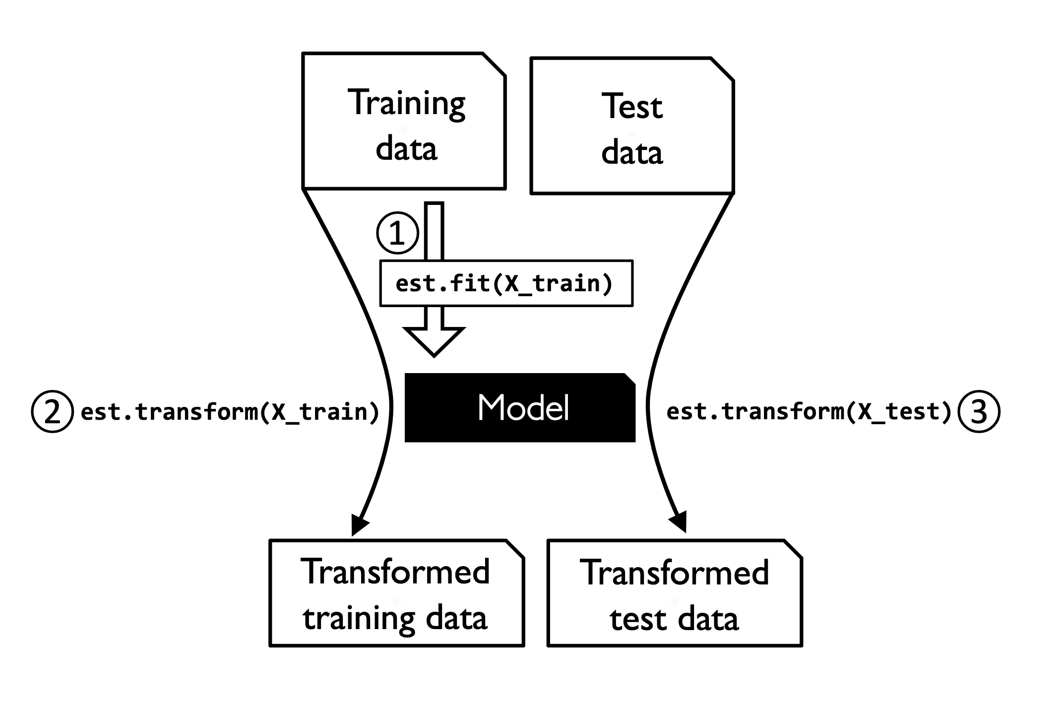
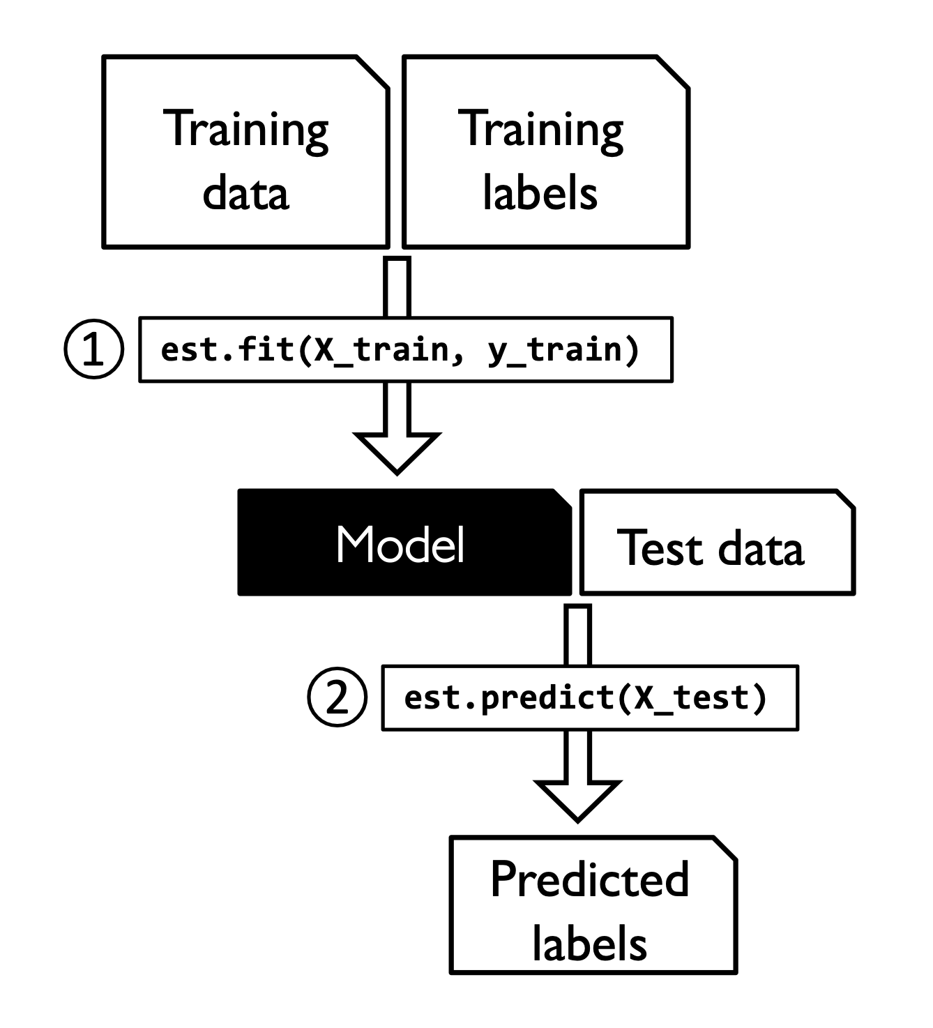
Understanding the scikit-learn estimator API¶

Handling categorical data¶

Nominal and ordinal features¶

This code creates a Pandas dataframe from a list of lists, where each list represents a row in the dataframe. The dataframe contains information about a set of items, with columns for ‘color’, ‘size’, ‘price’, and ‘classlabel’. The columns are given names using the .columns attribute of the dataframe. The resulting dataframe is then stored in the variable df.

Mapping ordinal features¶

This code creates a dictionary called size_mapping that maps the string values ‘XL’, ‘L’, and ‘M’ to integers 3, 2, and 1, respectively. The code then uses the map method from the Pandas DataFrame df to replace the values in the ‘size’ column with the corresponding integers in the size_mapping dictionary.

For example, the first row of the ‘size’ column has the value ‘M’, so it will be replaced with 1. The second row has the value ‘L’, so it will be replaced with 2, and so on. The modified DataFrame df is then displayed at the end of the code.

The line df['size'].map(inv_size_mapping) maps the numerical values back to the original categorical values using the ‘inv_size_mapping’ dictionary, which is created using the line inv_size_mapping = {v: k for k, v in size_mapping.items()} by swapping the keys and values of the ‘size_mapping’ dictionary.

Encoding class labels¶

This code is creating a dictionary called class_mapping that maps the unique class labels in the classlabel column of the DataFrame df to integers. The np.unique function is used to extract the unique class labels from the classlabel column. The enumerate function is used to generate a sequence of pairs, where the first element of each pair is an index, and the second element of each pair is a class label. The resulting dictionary maps each class label to a unique integer.

This code uses the map method of a Pandas DataFrame column, which applies a given mapping to each element in the column. In this case, the classlabel column is being transformed from strings to integers, using the class_mapping dictionary that was created earlier. The class_mapping dictionary maps each unique string class label in the classlabel column to an integer index, which is stored as the corresponding value in the dictionary.

The code below is using the LabelEncoder class from the sklearn.preprocessing module to perform label encoding on the class labels stored in the column 'classlabel' of the pandas DataFrame df.

The fit_transform method of the LabelEncoder class is used to fit the label encoder to the class labels and then perform the transformation to convert the class labels from strings to integers. The transformed integer representation of the class labels is stored in the variable y.

Performing one-hot encoding on nominal features¶

This code is preprocessing the data by converting the categorical feature “color” into numerical values. The LabelEncoder class from the sklearn.preprocessing library is used for this purpose.

First, the feature data is extracted from the Pandas dataframe df into a NumPy array X. The first column of X, which corresponds to the “color” feature, is then transformed using the fit_transform method of the LabelEncoder class. This method fits the encoder to the categorical feature data and returns a transformed array of numerical values.

After the transformation, the first column of X now contains numerical values that represent the categorical feature “color”.

This code performs one-hot encoding on the first column of the feature matrix X (which is the ‘color’ column) using the OneHotEncoder class from scikit-learn. The purpose of one-hot encoding is to transform categorical features, which are represented as integers, into a binary matrix representation.

The fit_transform method of the OneHotEncoder class takes in a 2D array as input, so we reshape the 1D array X[:, 0] into a 2D array X[:, 0].reshape(-1, 1) to make sure it fits the input format of the fit_transform method. The toarray method is used to convert the sparse matrix returned by the fit_transform method into a dense NumPy array.

This code uses ColumnTransformer from scikit-learn to apply different preprocessing techniques to different columns in the input feature array X. The ColumnTransformer takes a list of transformers as argument, where each transformer is defined by a name, an instance of a transformer class, and a list of indices specifying which columns to apply the transformer to. In this case, the first transformer is an instance of OneHotEncoder and is applied to the first column of X (the color feature). The second transformer is specified as 'nothing' with 'passthrough' as the class and is applied to the second and third columns of X (the size and price features, respectively). The ColumnTransformer applies the specified transformers to the columns in X and returns the transformed array. The resulting array is then cast to float type using astype(float).

The code is creating a one-hot encoding of the data in the df dataframe for the columns 'price', 'color', and 'size' using pandas’ get_dummies function. One-hot encoding is a process of converting categorical variables into a numerical representation, where each category value is represented as a separate binary column (also known as a “dummy variable”). The new columns created by the get_dummies function are binary columns, each representing one category of the original categorical column. The get_dummies function returns the transformed data as a new dataframe, which can be used for machine learning tasks.

The drop_first parameter in pd.get_dummies is used to prevent multicollinearity. Multicollinearity is a phenomenon in which two or more predictors in a regression model are highly correlated, causing the coefficients to become unstable. In the one-hot encoding process, the first category of a categorical variable is dropped to avoid the dummy variable trap, which is another way to prevent multicollinearity. By setting drop_first=True, the first category of each categorical variable is dropped from the encoding process, reducing the number of columns in the resulting dataframe. This can also help to reduce the risk of overfitting, as it reduces the number of predictors in the model.

This code is using the OneHotEncoder method from the scikit-learn library to perform one-hot encoding on the “color” feature in the input data X. The input data X is a matrix or 2D array-like object with three columns (features), and the OneHotEncoder will transform the first column (index 0) into multiple columns, one for each unique category in that column.

The code also uses the ColumnTransformer class from scikit-learn, which allows you to apply different transformations to different columns of your input data. In this case, the ColumnTransformer is being used to apply the one-hot encoding transformation only to the “color” feature (column 0), while leaving the other two features unchanged.

The OneHotEncoder is instantiated with two parameters: “categories=‘auto’” means that the categories to encode should be automatically inferred from the input data, and “drop=‘first’” means that the first category in each feature should be dropped to reduce multicollinearity.

Finally, the fit_transform method of the ColumnTransformer is used to fit the one-hot encoder to the input data and then transform the data. The resulting transformed data is then cast to type float to ensure that all values are numerical.

Optional: Encoding Ordinal Features¶

If we are unsure about the numerical differences between the categories of ordinal features, or the difference between two ordinal values is not defined, we can also encode them using a threshold encoding with 0/1 values. For example, we can split the feature “size” with values M, L, and XL into two new features “x > M” and “x > L”. Let’s consider the original DataFrame:

We can use the apply method of pandas’ DataFrames to write custom lambda expressions in order to encode these variables using the value-threshold approach:

Partitioning a dataset into a separate training and test set¶

This code is a demonstration of how to split a dataset into training and testing sets using the train_test_split function from the sklearn.model_selection module in scikit-learn.

The first line extract the feature values and target values from the df_wine dataframe into X and y respectively.

In the next line, the train_test_split function is used to split X and y into training and testing sets. The function takes several parameters:

• X and y: the feature values and target values that we want to split.

• test_size: the proportion of the data that should be allocated to the test set. In this case, 0.3 means that 30% of the data will be allocated to the test set and 70% to the training set.

• random_state: a seed for the random number generator used to shuffle the data before splitting it. This makes the split reproducible.

• stratify: This ensures that the proportion of each target class is approximately the same in both the training and test sets.

Bringing features onto the same scale¶

This code applies the MinMaxScaler method from the scikit-learn library to scale the features of the training set X_train and the test set X_test. The MinMaxScaler method scales each feature to a given range, usually [0, 1]. The fit_transform method is used to fit the scaler to the training set and also return the transformed training set. The transform method is then used to apply the same scaling parameters to the test set, so that both the training set and the test set are transformed with the same scaling parameters. This is important so that the comparison between the predicted values and the true values in the test set is fair, as both the inputs and the outputs are scaled in the same way.

The code imports the StandardScaler class from scikit-learn’s preprocessing module. The StandardScaler performs standardization on the input data, transforming it so that it has a mean of 0 and a standard deviation of 1.

Here, a StandardScaler object stdsc is created and then fit_transform method is called on the training data X_train to fit the stdsc object to the data and transform the training data to have a mean of 0 and a standard deviation of 1. The same stdsc object is then used to transform the test data X_test with the transform method.

This is different from MinMaxScaler in the sense that MinMaxScaler scales the data to a specific range (typically 0 to 1), whereas StandardScaler standardizes the data so it has a mean of 0 and a standard deviation of 1.

A visual example:

Selecting meaningful features¶

...

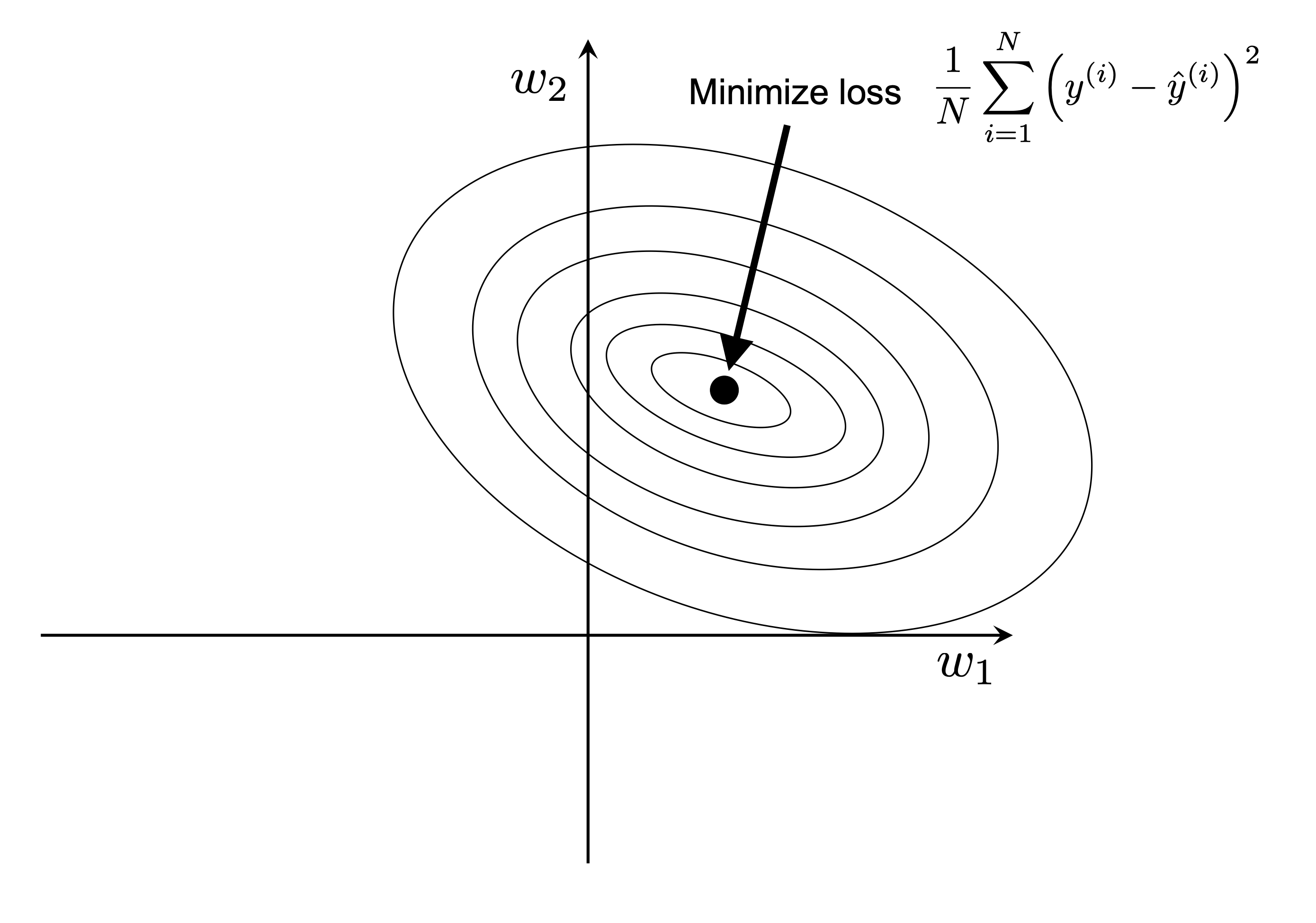
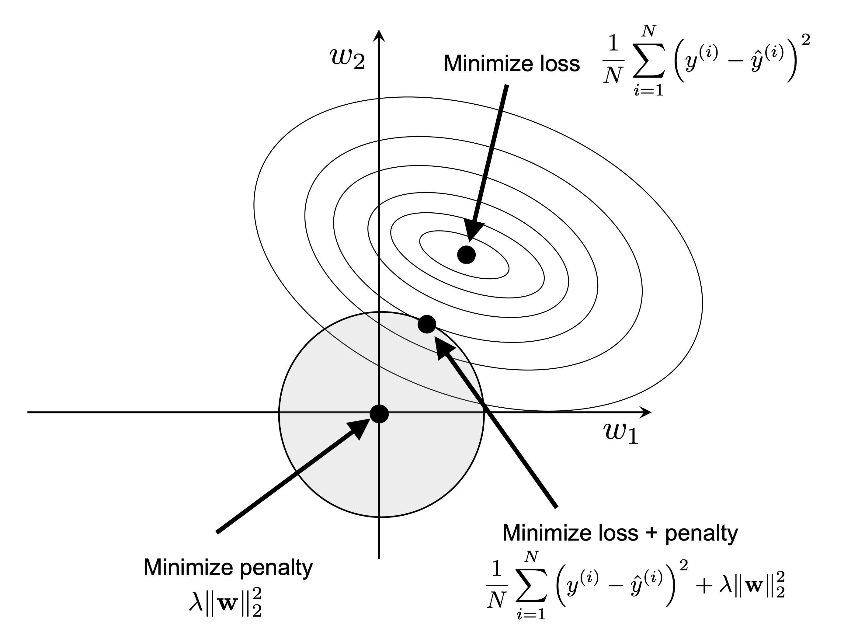
L1 and L2 regularization as penalties against model complexity¶

A geometric interpretation of L2 regularization¶

Sparse solutions with L1-regularization¶

For regularized models in scikit-learn that support L1 regularization, we can simply set the penalty parameter to 'l1' to obtain a sparse solution:

This code imports the Logistic Regression class from the scikit-learn library.

The LogisticRegression class is initialized with a penalty parameter, which determines the type of regularization that is applied to the model. In this code, the penalty parameter is set to ‘l1’, which means that L1 regularization will be used. L1 regularization is a technique that adds a penalty term to the loss function that the model is trying to minimize. The penalty term is proportional to the absolute values of the coefficients of the features in the model. This has the effect of shrinking the magnitude of the coefficients of unimportant features towards zero, effectively reducing the dimensionality of the feature space and making the model simpler.

So, this code creates a logistic regression model with L1 regularization, which can be useful in reducing overfitting and improving the interpretability of the model.

Applied to the standardized Wine data ...

This code imports the LogisticRegression class from the scikit-learn’s linear_model module. It then creates an instance of the LogisticRegression class and assigns it to the variable lr. The instance is configured with the L1 regularization penalty and a regularization strength of 1.0 (controlled by the C parameter). The solver liblinear is used for optimization and the multi_class parameter is set to ovr to handle the case of multiclass classification.

The fit method is then called on the lr object to fit the logistic regression model to the training data. The accuracy of the model is computed on both the training data and the test data using the score method and the results are printed.

The lr.intercept_ attribute in this code represents the bias of the logistic regression model. Bias, also known as the intercept, is a term used in machine learning to describe the constant term that is added to the linear combination of features to make predictions. In this example, since we are using the one-versus-rest (OVR) multi-class strategy, we have three separate logistic regression models, each with its own bias term, to handle the three wine classes in the dataset. This means that for a given example, each of the three models will make a prediction, and the class label with the highest predicted probability will be chosen as the final prediction.

np.set_printoptions(8) is a line of code that sets the print options for NumPy arrays. The number “8” inside the parentheses determines the number of digits of precision to display when printing the values in a NumPy array. By setting this value to “8”, we ensure that when we print NumPy arrays, they will be displayed with 8 digits of precision.

The lr.coef_ attribute returns the coefficients of the logistic regression model that correspond to each input feature. The code lr.coef_[lr.coef_!=0].shape is checking the shape of the coefficients that are not equal to zero. This is essentially counting the number of non-zero coefficients and returning the result as a tuple with one element, the number of non-zero coefficients. This can give us an idea of how many features the model is using and whether some features are being discarded by the L1 regularization.

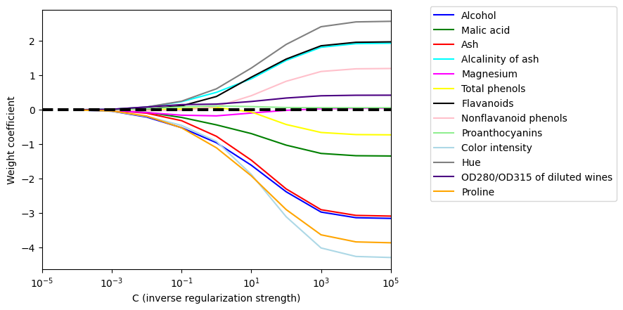
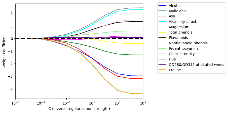
This script demonstrates the effect of L1 regularization on feature selection in a logistic regression model. L1 regularization is a technique that can be used to reduce the complexity of a model by setting some of the weight coefficients to zero, effectively removing those features from the model (embedded feature selection tehcnique). This can be useful for improving model performance and reducing overfitting.

The script then creates a logistic regression model with L1 regularization for a range of values of the regularization strength parameter C, and fits the model to the preprocessed data. For each value of C, the script appends the weight coefficients and regularization strength to separate lists.

The script then creates a plot showing the weight coefficients for each feature as a function of the regularization strength parameter C.

The script creates a plot that visualizes the change in weight coefficients for each feature as the regularization strength is varied, with each feature plotted as a separate line in a different color. A legend is added to the plot to help identify which feature each line corresponds to. The visualization shows that as the regularization strength is increased (i.e., as C is decreased), the L1 regularization technique shrinks the weight coefficients of some of the features towards zero. This has the effect of reducing the impact of those features on the model and can be used as a technique for feature selection.

Sequential feature selection algorithms¶

This code defines a class called SBS (sequential backward selection) which is a feature selection technique for machine learning models. The class can be used to select a subset of features from a dataset that will produce a good performing model.

The SBS class has two main methods: fit() and transform(). The fit() method takes a dataset as input and performs sequential backward selection on the features, reducing the number of features until the specified number of features is reached. The method outputs the indices of the selected features.

The transform() method takes the dataset as input and returns the selected subset of features.

The SBS class uses a provided estimator (classifier or regression model) to fit the data and a provided scoring function to evaluate the performance of the estimator. The method starts with all the features and iteratively removes the least important feature until the specified number of features is reached.

The SBS class first splits the dataset into training and testing sets using train_test_split() from scikit-learn. The method then initializes a set of indices corresponding to all the features and the set of subsets containing all the indices. The method then calculates the score of the model using the scoring function provided.

The method then loops through each feature and removes it from the feature set to create a new subset of features. The score of the new subset is calculated and stored in a list. This process is repeated until the desired number of features is reached.

The SBS class keeps track of the best subset of features selected and the corresponding score. Finally, the method outputs the subset of features that achieved the best score.

In summary, the SBS class is a useful tool for feature selection in machine learning, providing a systematic way to remove features from a dataset and select the best subset for a model.

This code demonstrates how to use the SBS (sequential backward selection) class to select a subset of features from a dataset and evaluate the performance of a K-Nearest Neighbor (KNN) classifier on the selected subset.

First, a KNN classifier with five neighbors is initialized using KNeighborsClassifier(n_neighbors=5).

Next, the SBS class is used to select a subset of features from the standardized training dataset X_train_std and the corresponding labels y_train. The fit() method of the SBS class is used to fit the KNN classifier to the training data and perform sequential backward selection to reduce the number of features until the desired number of features (one in this case) is reached. The resulting best subset of features is stored in the sbs.subsets_ attribute of the SBS class.

Finally, a plot is created to show how the performance of the KNN classifier varies as the number of selected features is increased. The number of features in each subset is stored in the k_feat list, and the accuracy of the KNN classifier on each subset is stored in the sbs.scores_ list. The plt.plot() function is used to plot the accuracy as a function of the number of features, and various formatting functions are used to adjust the appearance of the plot.

Overall, this code provides a useful example of how to use the SBS class to select a subset of features and evaluate the performance of a machine learning model on the selected subset. The resulting plot can be used to identify the optimal number of features to use for the KNN classifier.

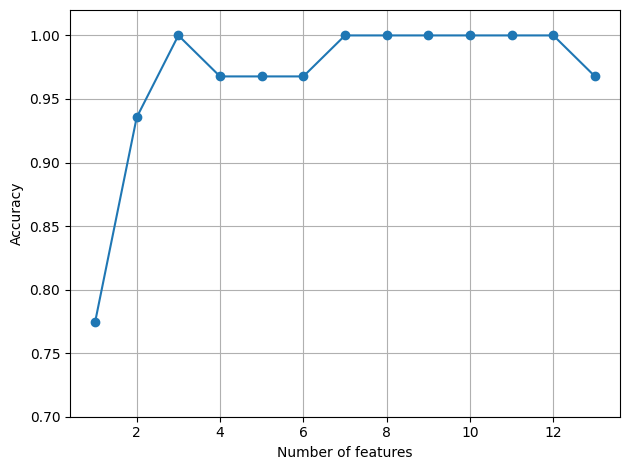
This code prints the names of the features that were selected by the SBS (sequential backward selection) class.

The code selects the 11th subset of features from the sbs.subsets_ attribute of the SBS class, which represents the set of features selected when only 3 features remain. The indices of the selected features are stored in the k3 list.

The df_wine.columns[1:] expression is used to get the names of the features, excluding the target variable column. The k3 list is then used to select the names of the features that were selected by the SBS class.

Finally, the names of the selected features are printed to the console.

In summary, this code provides a way to determine which features were selected by the SBS class, which can be useful for understanding which features are most important for the KNN classifier.

Example¶

Comparing different feature seleciton technique from sciki-learn

Assessing feature importance with Random Forests¶

This code demonstrates how to use a random forest classifier to estimate the importance of each feature in a dataset.

First, the names of the features in the Wine dataset are assigned to the feat_labels variable.

Next, a random forest classifier is initialized with 500 trees and a random state of 1 using RandomForestClassifier(n_estimators=500, random_state=1). The classifier is then fit to the training data X_train and the corresponding labels y_train using the fit() method.

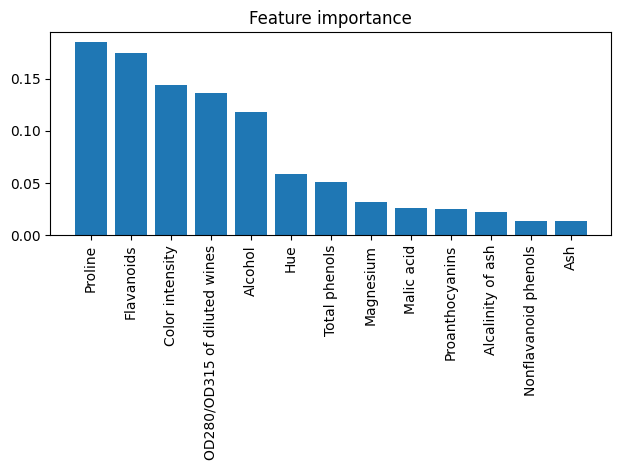
The feature_importances_ attribute of the random forest classifier is used to estimate the importance of each feature in the dataset. The np.argsort() function is used to sort the features in descending order of importance, and the sorted indices are stored in the indices variable.

Finally, a plot is created to visualize the feature importances. The plt.bar() function is used to create a horizontal bar plot of the feature importances, and the plt.xticks() function is used to label each bar with the corresponding feature name. The plot provides a visual representation of the importance of each feature, with more important features having larger bars.

Overall, this code is a useful example of how to use a random forest classifier to estimate feature importances and create a plot to visualize the results. The resulting plot can be used to identify which features are most important for the classifier and can be used to guide feature selection or engineering efforts.

This code demonstrates how to use the SelectFromModel class from scikit-learn to select a subset of features from a dataset based on a threshold of feature importance.

First, the SelectFromModel class is imported from scikit-learn using from sklearn.feature_selection.

Next, the SelectFromModel class is initialized with the random forest classifier forest as the estimator and a threshold of 0.1 for feature selection. The prefit parameter is set to True, which indicates that the estimator has already been fit to the data.

The transform() method of the SelectFromModel class is used to transform the training data X_train to the selected subset of features based on the feature importances calculated by the random forest classifier. The resulting subset of features is stored in the X_selected variable.

Finally, the number of features in the selected subset is printed to the console using X_selected.shape[1].

In summary, this code demonstrates how to use the SelectFromModel class to select a subset of features based on a threshold of feature importance, which can be a useful technique for reducing the dimensionality of a dataset and improving the performance of machine learning models.

Now, let’s print the 5 features that met the threshold criterion for feature selection that we set earlier (note that this code snippet does not appear in the actual book but was added to this notebook later for illustrative purposes):

Summary¶

...

Readers may ignore the next cell.