

Training Simple Machine Learning Algorithms for Classification
Annotated chapter code — Dr. Brian Jalaian
Package version checks
Add folder to path in order to load from the check_packages.py script:
import sys
sys.path.insert(0, '..')  # kept for compatibility; not required on Colab
Check recommended package versions:
# Package version check (Colab-safe: no external script required)
import importlib

def check_packages(d):
    for pkg_name, min_version in d.items():
        try:
            imported = importlib.import_module(pkg_name)
            version = getattr(imported, '__version__', 'unknown')
            print(f'[OK] {pkg_name} {version}')
        except ImportError:
            print(f'[MISSING] {pkg_name} is not installed')

d = {
    'numpy': '1.21.2',
    'matplotlib': '3.4.3',
    'pandas': '1.3.2'
}
check_packages(d)
[OK] numpy 2.0.2
[OK] matplotlib 3.10.0
[OK] pandas 2.2.2
Chapter 2 - Training Machine Learning Algorithms for Classification
Overview
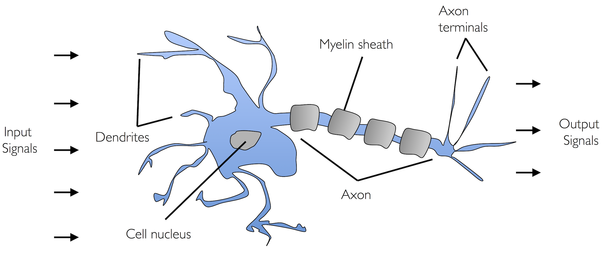
from IPython.display import ImageArtificial neurons - a brief glimpse into the early history of machine learning
import os, urllib.request
os.makedirs('figures', exist_ok=True)
fig_path = 'figures/02_01.png'
if not os.path.exists(fig_path):
    url = 'https://raw.githubusercontent.com/rasbt/machine-learning-book/main/ch02/figures/02_01.png'
    try:
        urllib.request.urlretrieve(url, fig_path)
    except Exception as e:
        print(f'Could not download figure: {e}')
if os.path.exists(fig_path):
    display(Image(filename=fig_path, width=500))
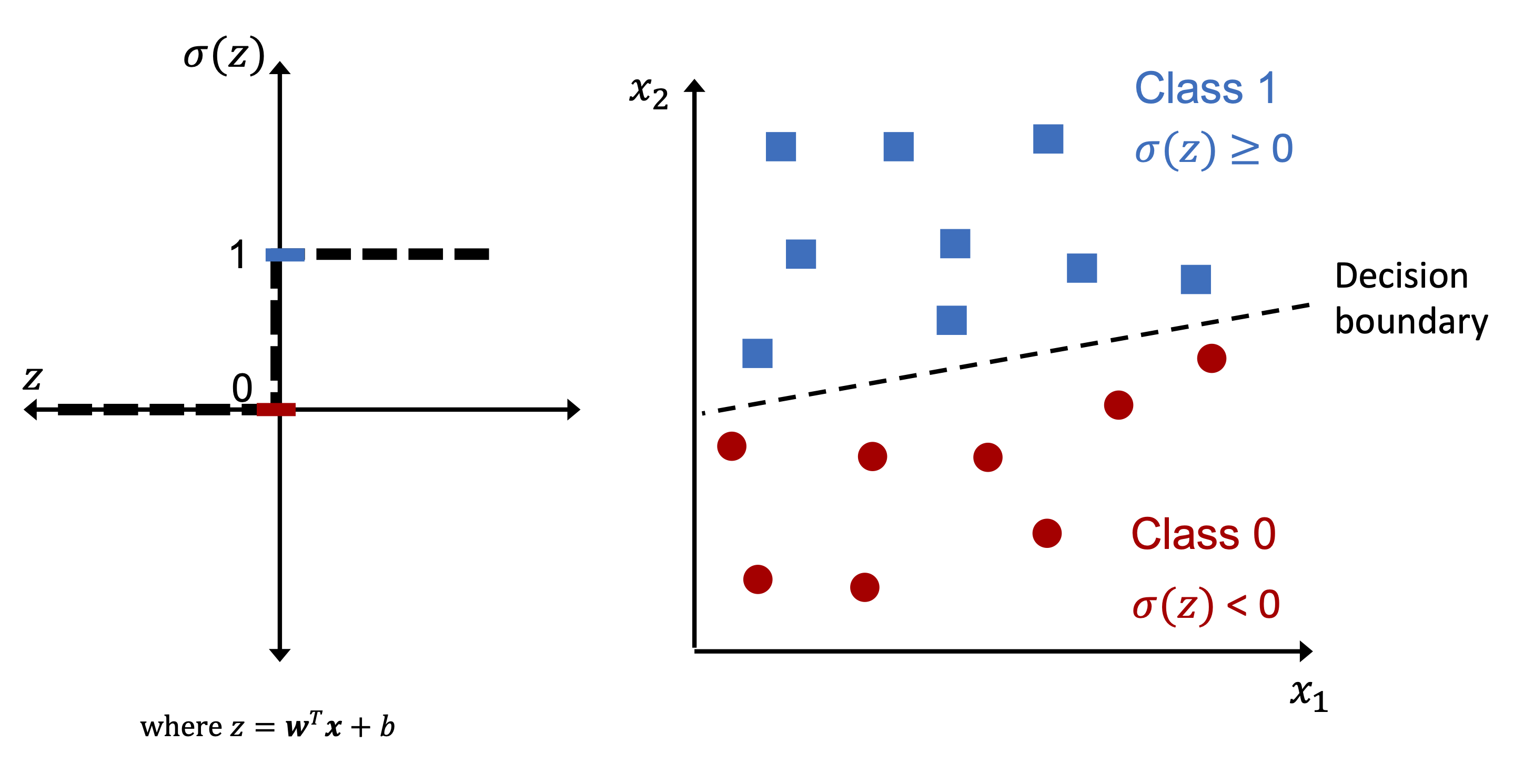
The formal definition of an artificial neuron
import os, urllib.request
os.makedirs('figures', exist_ok=True)
fig_path = 'figures/02_02.png'
if not os.path.exists(fig_path):
    url = 'https://raw.githubusercontent.com/rasbt/machine-learning-book/main/ch02/figures/02_02.png'
    try:
        urllib.request.urlretrieve(url, fig_path)
    except Exception as e:
        print(f'Could not download figure: {e}')
if os.path.exists(fig_path):
    display(Image(filename=fig_path, width=600))
The perceptron learning rule
import os, urllib.request
os.makedirs('figures', exist_ok=True)
fig_path = 'figures/02_03.png'
if not os.path.exists(fig_path):
    url = 'https://raw.githubusercontent.com/rasbt/machine-learning-book/main/ch02/figures/02_03.png'
    try:
        urllib.request.urlretrieve(url, fig_path)
    except Exception as e:
        print(f'Could not download figure: {e}')
if os.path.exists(fig_path):
    display(Image(filename=fig_path, width=600))
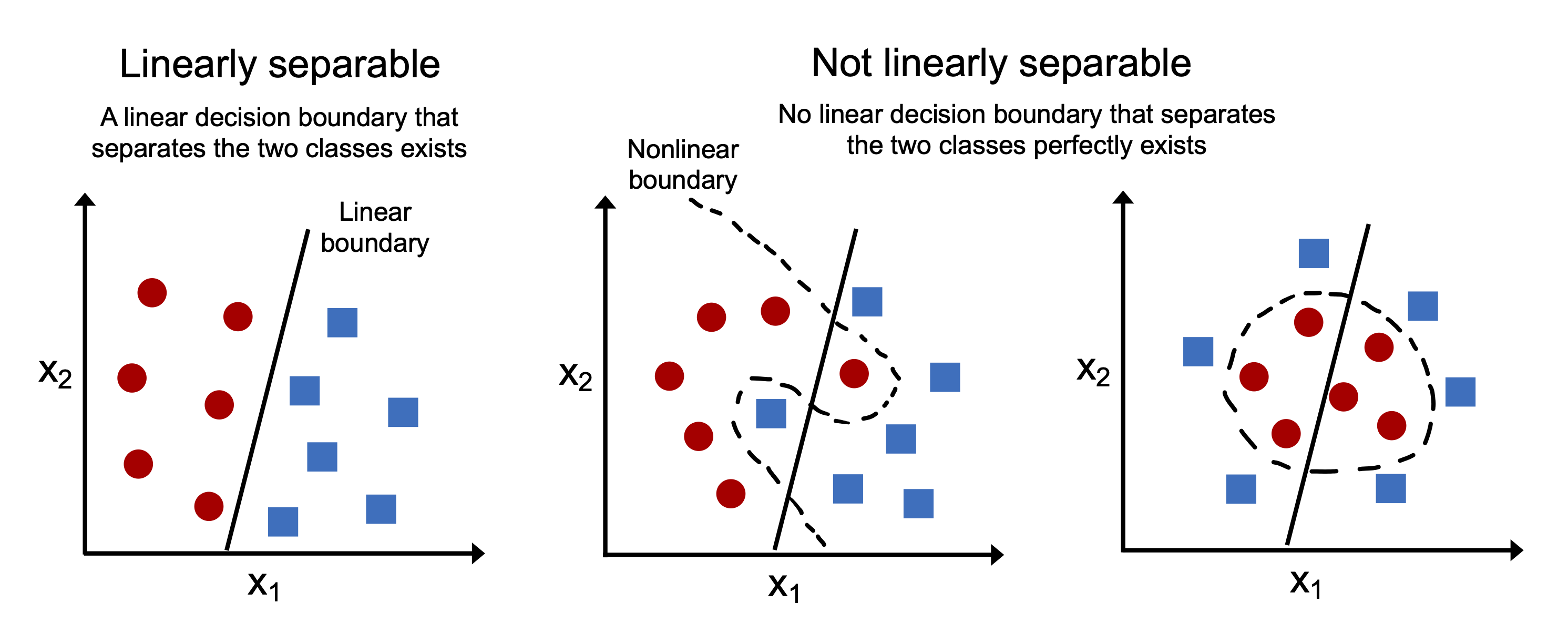
import os, urllib.request
os.makedirs('figures', exist_ok=True)
fig_path = 'figures/02_04.png'
if not os.path.exists(fig_path):
    url = 'https://raw.githubusercontent.com/rasbt/machine-learning-book/main/ch02/figures/02_04.png'
    try:
        urllib.request.urlretrieve(url, fig_path)
    except Exception as e:
        print(f'Could not download figure: {e}')
if os.path.exists(fig_path):
    display(Image(filename=fig_path, width=600))
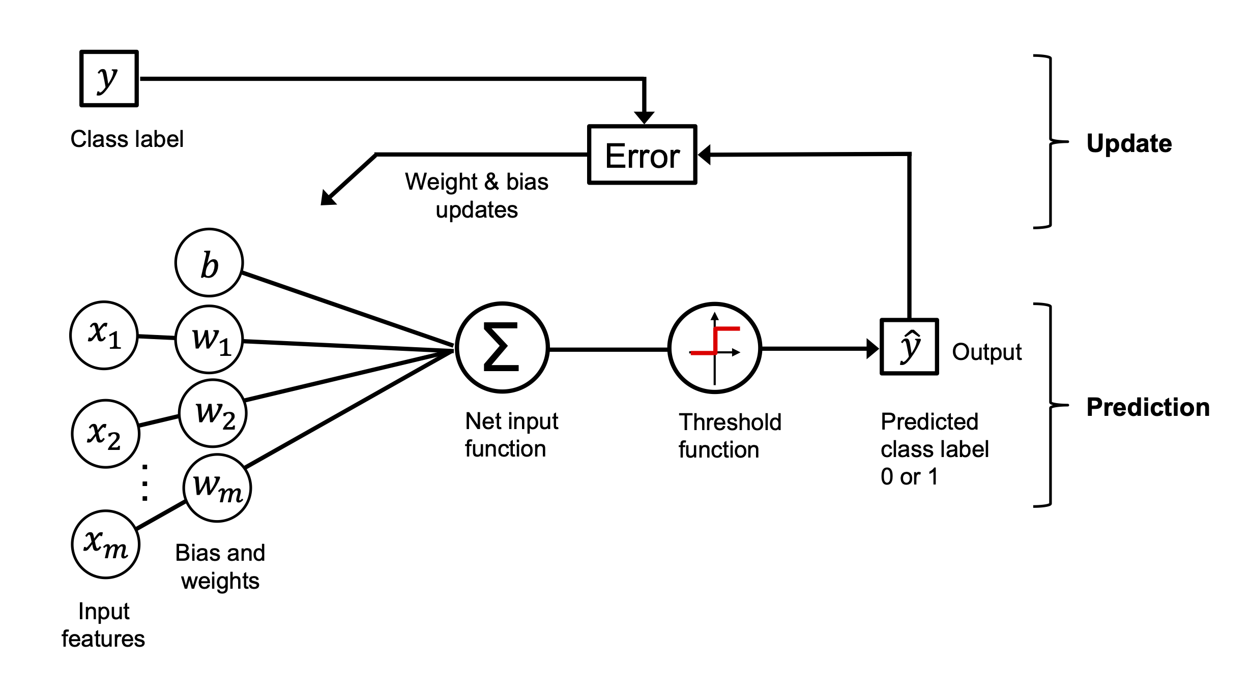
Implementing a perceptron learning algorithm in Python
An object-oriented perceptron API
This code defines a Python class called Perceptron which implements the perceptron algorithm for binary classification. The class has several methods, including init, fit, net_input, and predict.
The init method is the constructor for the class. It sets the initial values for the learning rate (eta), the number of passes over the training dataset (n_iter), and the random number generator seed for initializing the weights (random_state).
The fit method is used to train the perceptron model. It takes in the training data and target values, and updates the weights and bias unit until convergence or the maximum number of iterations is reached. The number of misclassifications in each iteration is stored in the errors_ list attribute.
The net_input method calculates the dot product of the input data and weights, plus the bias unit.
The predict method takes in input data and returns the predicted class label using the np.where function, which returns 1 if the net input is greater than or equal to 0, and 0 otherwise.
It is worth noting that, this particular implementation is a simple version of the perceptron and it does not account for non-linearly separable datasets, for which more sophisticated linear classifiers like the SVM or Logistic Regression should be used.
import numpy as np


class Perceptron:
    """Perceptron classifier.

    Parameters
    ------------
    eta : float
      Learning rate (between 0.0 and 1.0)
    n_iter : int
      Passes over the training dataset.
    random_state : int
      Random number generator seed for random weight
      initialization.

    Attributes
    -----------
    w_ : 1d-array
      Weights after fitting.
    b_ : Scalar
      Bias unit after fitting.
    errors_ : list
      Number of misclassifications (updates) in each epoch.

    """
    def __init__(self, eta=0.01, n_iter=50, random_state=1):
        self.eta = eta
        self.n_iter = n_iter
        self.random_state = random_state

    def fit(self, X, y):
        """Fit training data.

        Parameters
        ----------
        X : {array-like}, shape = [n_examples, n_features]
          Training vectors, where n_examples is the number of examples and
          n_features is the number of features.
        y : array-like, shape = [n_examples]
          Target values.

        Returns
        -------
        self : object

        """
        rgen = np.random.RandomState(self.random_state)
        self.w_ = rgen.normal(loc=0.0, scale=0.01, size=X.shape[1])
        self.b_ = np.float64(0.)

        self.errors_ = []

        for _ in range(self.n_iter):
            errors = 0
            for xi, target in zip(X, y):
                update = self.eta * (target - self.predict(xi))
                self.w_ += update * xi
                self.b_ += update
                errors += int(update != 0.0)
            self.errors_.append(errors)
        return self

    def net_input(self, X):
        """Calculate net input"""
        return np.dot(X, self.w_) + self.b_

    def predict(self, X):
        """Return class label after unit step"""
        return np.where(self.net_input(X) >= 0.0, 1, 0)
Training a perceptron model on the Iris dataset
...
Reading-in the Iris data
import os
import pandas as pd
from urllib.error import HTTPError, URLError

try:
    s = 'https://archive.ics.uci.edu/ml/machine-learning-databases/iris/iris.data'
    print('From URL:', s)
    df = pd.read_csv(s, header=None, encoding='utf-8')
except (HTTPError, URLError, Exception) as e:
    # Fall back to the book's GitHub-hosted copy of the Iris dataset,
    # since the UCI server is sometimes unavailable / blocks automated requests.
    s = 'https://raw.githubusercontent.com/rasbt/machine-learning-book/main/ch02/iris.data'
    print('UCI source failed ({}), falling back to:'.format(e), s)
    df = pd.read_csv(s, header=None, encoding='utf-8')

df.tail()
From URL: https://archive.ics.uci.edu/ml/machine-learning-databases/iris/iris.data
Plotting the Iris data
The code uses the matplotlib and numpy libraries to plot a scatter plot of sepal length and petal length for two classes of iris flower species: Setosa and Versicolor. The data is loaded from a DataFrame df, and the first 100 rows of the data are selected. The y variable is set to be the species column of the data, where ‘Iris-setosa’ is labeled as 0 and ‘Iris-versicolor’ is labeled as 1. The X variable is set to be the sepal length and petal length columns of the data. The code uses the scatter function to plot the data, where Setosa data points are plotted as red circles and Versicolor data points are plotted as blue squares. The x-axis is labeled as ‘Sepal length [cm]’ and the y-axis is labeled as ‘Petal length [cm]’, and a legend is added to the upper left corner of the plot to show the class labels. Finally, the show function is called to display the plot.
#%matplotlib inline
import matplotlib.pyplot as plt
import numpy as np

# select setosa and versicolor
y = df.iloc[0:100, 4].values
y = np.where(y == 'Iris-setosa', 0, 1)

# extract sepal length and petal length
X = df.iloc[0:100, [0, 2]].values

# plot data
plt.scatter(X[:50, 0], X[:50, 1],
            color='red', marker='o', label='Setosa')
plt.scatter(X[50:100, 0], X[50:100, 1],
            color='blue', marker='s', label='Versicolor')

plt.xlabel('Sepal length [cm]')
plt.ylabel('Petal length [cm]')
plt.legend(loc='upper left')

# plt.savefig('images/02_06.png', dpi=300)
plt.show()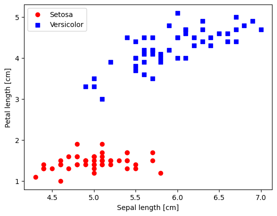
Training the perceptron model
This code creates an instance of the Perceptron class with a learning rate of 0.1 and 10 iterations. The fit method is then called on the instance with the variables X and y as the parameters, where X represents the feature variables and y represents the target variable. The plot method is then used to create a graph with the x-axis representing the number of iterations and the y-axis representing the number of updates (misclassifications) during each iteration. This graph helps to visualize the learning process of the perceptron algorithm and its convergence.
ppn = Perceptron(eta=0.1, n_iter=10)

ppn.fit(X, y)

plt.plot(range(1, len(ppn.errors_) + 1), ppn.errors_, marker='o')
plt.xlabel('Epochs')
plt.ylabel('Number of updates')

# plt.savefig('images/02_07.png', dpi=300)
plt.show()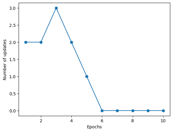
A function for plotting decision regions
The function plot_decision_regions takes as inputs:
X : a 2D array with shape (n_examples, n_features) representing the feature vectors of the input dataset
y : a 1D array with shape (n_examples,) representing the target values
classifier : the classifier object that has already been fit to the data
resolution : a float value that will be used to control the granularity of the grid used to generate the decision regions
The function creates a scatter plot of the input dataset, where each class is represented by a different marker and color, and overlays the decision regions of the classifier on top of it.
The following steps are performed:
Create markers and colors for the different classes
Create a grid of points on the feature space, using the minimum and maximum values of each feature and the specified resolution.
Use the classifier to predict the class of each point on the grid.
Plot the decision regions, using the grid points and their predicted classes.
Plot the input data points, using the markers and colors created in step 1
from matplotlib.colors import ListedColormap


def plot_decision_regions(X, y, classifier, resolution=0.02):

    # setup marker generator and color map
    markers = ('o', 's', '^', 'v', '<')
    colors = ('red', 'blue', 'lightgreen', 'gray', 'cyan')
    cmap = ListedColormap(colors[:len(np.unique(y))])

    # plot the decision surface
    x1_min, x1_max = X[:, 0].min() - 1, X[:, 0].max() + 1
    x2_min, x2_max = X[:, 1].min() - 1, X[:, 1].max() + 1
    xx1, xx2 = np.meshgrid(np.arange(x1_min, x1_max, resolution),
                           np.arange(x2_min, x2_max, resolution))
    lab = classifier.predict(np.array([xx1.ravel(), xx2.ravel()]).T)
    lab = lab.reshape(xx1.shape)
    plt.contourf(xx1, xx2, lab, alpha=0.3, cmap=cmap)
    plt.xlim(xx1.min(), xx1.max())
    plt.ylim(xx2.min(), xx2.max())

    # plot class examples
    for idx, cl in enumerate(np.unique(y)):
        plt.scatter(x=X[y == cl, 0],
                    y=X[y == cl, 1],
                    alpha=0.8,
                    c=colors[idx],
                    marker=markers[idx],
                    label=f'Class {cl}',
                    edgecolor='black')
plot_decision_regions(X, y, classifier=ppn)
plt.xlabel('Sepal length [cm]')
plt.ylabel('Petal length [cm]')
plt.legend(loc='upper left')
#plt.savefig('images/02_08.png', dpi=300)
plt.show()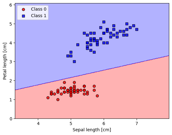
Adaptive linear neurons and the convergence of learning
...
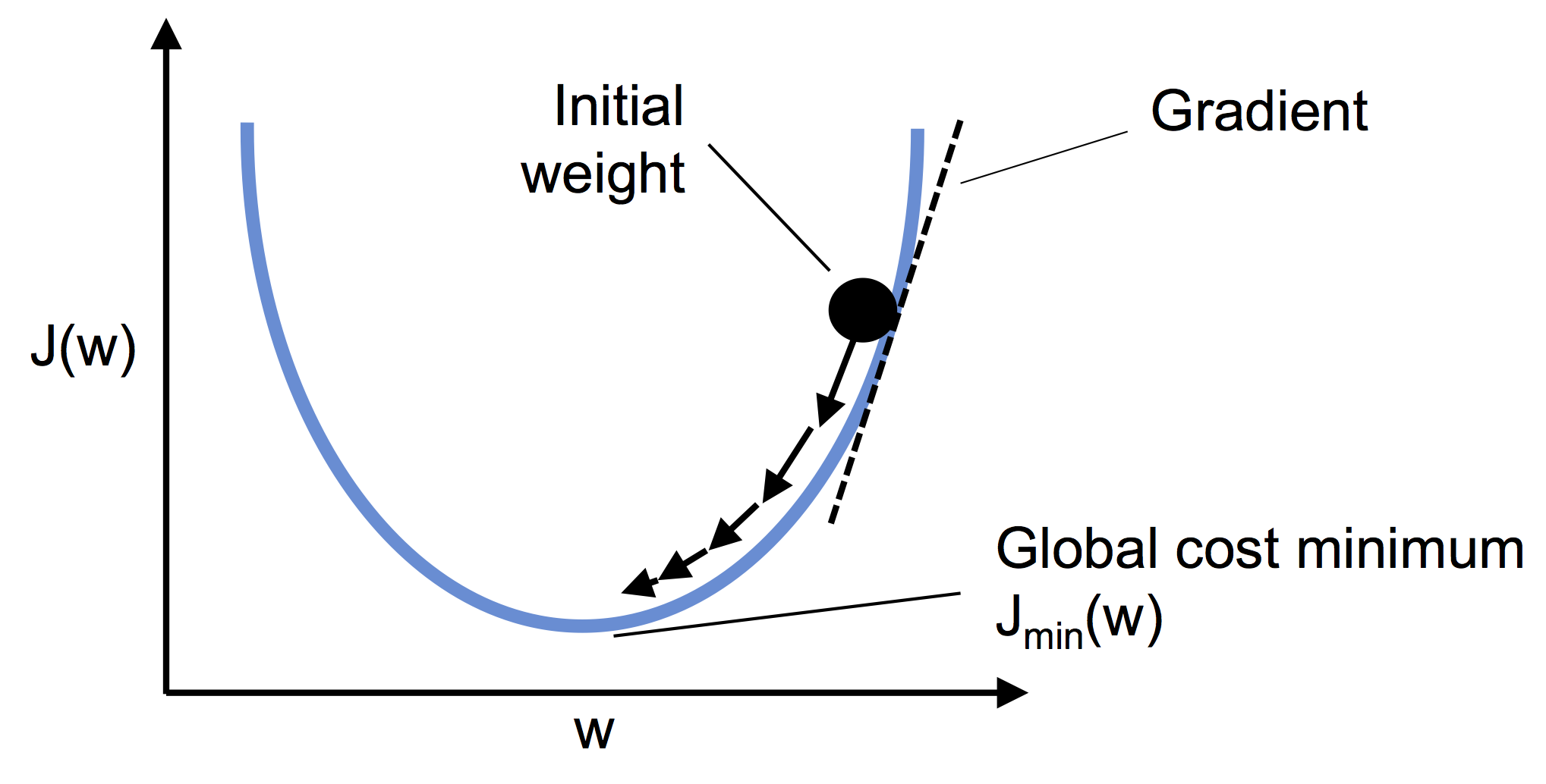
Minimizing cost functions with gradient descent
import os, urllib.request
os.makedirs('figures', exist_ok=True)
fig_path = 'figures/02_09.png'
if not os.path.exists(fig_path):
    url = 'https://raw.githubusercontent.com/rasbt/machine-learning-book/main/ch02/figures/02_09.png'
    try:
        urllib.request.urlretrieve(url, fig_path)
    except Exception as e:
        print(f'Could not download figure: {e}')
if os.path.exists(fig_path):
    display(Image(filename=fig_path, width=600))
import os, urllib.request
os.makedirs('figures', exist_ok=True)
fig_path = 'figures/02_10.png'
if not os.path.exists(fig_path):
    url = 'https://raw.githubusercontent.com/rasbt/machine-learning-book/main/ch02/figures/02_10.png'
    try:
        urllib.request.urlretrieve(url, fig_path)
    except Exception as e:
        print(f'Could not download figure: {e}')
if os.path.exists(fig_path):
    display(Image(filename=fig_path, width=500))
Implementing an adaptive linear neuron in Python
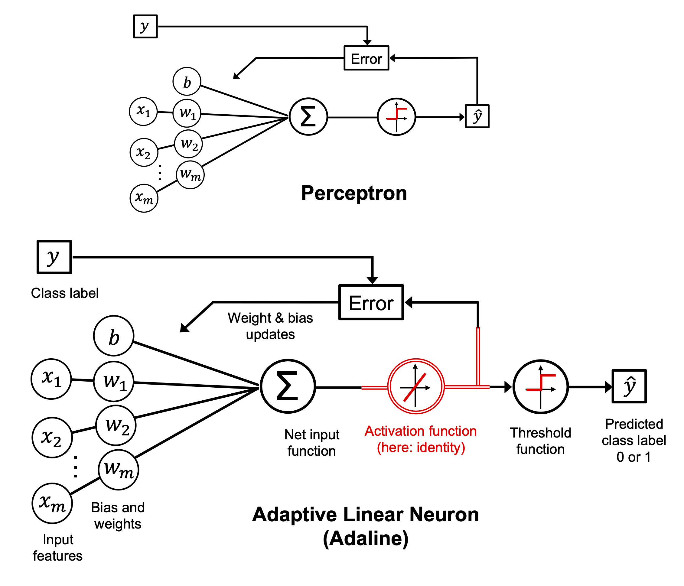
The AdalineGD class is an implementation of the Adaline algorithm, an adaptive linear neuron. The class has several methods and attributes, including:
__init__(self, eta=0.01, n_iter=50, random_state=1): This is the constructor method for the AdalineGD class. It initializes the learning rate (eta), number of iterations (n_iter), and random seed for weight initialization (random_state) with default values of 0.01, 50, and 1 respectively.fit(self, X, y): This method fits the training data (X) and the target values (y) to the model. It initializes the weights (w_) and bias (b_) with random values, and then iterates over the number of iterations specified in the constructor. In each iteration, it calculates the net input, computes the output using the activation function, and computes the error. The weights and bias are then updated based on these errors.net_input(self, X): This method calculates the net input by taking the dot product of the training data (X) and the weights (w_), and adding the bias (b_).activation(self, X): This method computes the linear activation, which is simply the identity function of the net input.predict(self, X): This method returns the class labels after applying the unit step function on the linear activation.
class AdalineGD:
    """ADAptive LInear NEuron classifier.

    Parameters
    ------------
    eta : float
      Learning rate (between 0.0 and 1.0)
    n_iter : int
      Passes over the training dataset.
    random_state : int
      Random number generator seed for random weight
      initialization.


    Attributes
    -----------
    w_ : 1d-array
      Weights after fitting.
    b_ : Scalar
      Bias unit after fitting.
    losses_ : list
      Mean squared eror loss function values in each epoch.

    """
    def __init__(self, eta=0.01, n_iter=50, random_state=1):
        self.eta = eta
        self.n_iter = n_iter
        self.random_state = random_state

    def fit(self, X, y):
        """ Fit training data.

        Parameters
        ----------
        X : {array-like}, shape = [n_examples, n_features]
          Training vectors, where n_examples is the number of examples and
          n_features is the number of features.
        y : array-like, shape = [n_examples]
          Target values.

        Returns
        -------
        self : object

        """
        rgen = np.random.RandomState(self.random_state)
        self.w_ = rgen.normal(loc=0.0, scale=0.01, size=X.shape[1])
        self.b_ = np.float64(0.)
        self.losses_ = []

        for i in range(self.n_iter):
            net_input = self.net_input(X)
            # Please note that the "activation" method has no effect
            # in the code since it is simply an identity function. We
            # could write `output = self.net_input(X)` directly instead.
            # The purpose of the activation is more conceptual, i.e.,
            # in the case of logistic regression (as we will see later),
            # we could change it to
            # a sigmoid function to implement a logistic regression classifier.
            output = self.activation(net_input)
            errors = (y - output)

            #for w_j in range(self.w_.shape[0]):
            #    self.w_[w_j] += self.eta * (2.0 * (X[:, w_j]*errors)).mean()

            self.w_ += self.eta * 2.0 * X.T.dot(errors) / X.shape[0]
            self.b_ += self.eta * 2.0 * errors.mean()
            loss = (errors**2).mean()
            self.losses_.append(loss)
        return self

    def net_input(self, X):
        """Calculate net input"""
        return np.dot(X, self.w_) + self.b_

    def activation(self, X):
        """Compute linear activation"""
        return X

    def predict(self, X):
        """Return class label after unit step"""
        return np.where(self.activation(self.net_input(X)) >= 0.5, 1, 0)
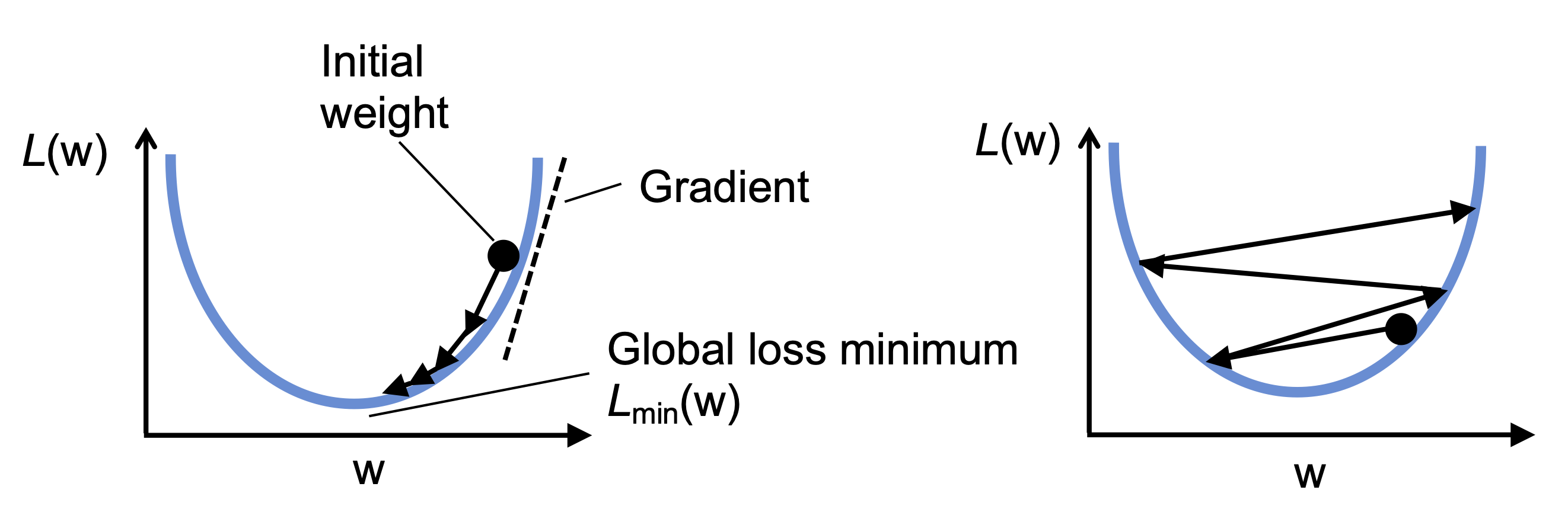
The following code creates two instances of the AdalineGD class, one with a learning rate of 0.1 and the other with a learning rate of 0.0001. Both instances are trained on the feature variables X and the target variable y using the fit method. The first instance is plotted on the left axis of a subplot, with the x-axis representing the number of epochs and the y-axis representing the logarithm of the mean squared error loss function. The second instance is plotted on the right axis of the same subplot, with the x-axis and y-axis representing the same as the first instance but with a linear scale instead of a logarithmic scale. This comparison helps to illustrate the effect of the learning rate on the convergence of the Adaline learning rule.
fig, ax = plt.subplots(nrows=1, ncols=2, figsize=(10, 4))

ada1 = AdalineGD(n_iter=15, eta=0.1).fit(X, y)
ax[0].plot(range(1, len(ada1.losses_) + 1), np.log10(ada1.losses_), marker='o')
ax[0].set_xlabel('Epochs')
ax[0].set_ylabel('log(Mean squared error)')
ax[0].set_title('Adaline - Learning rate 0.1')

ada2 = AdalineGD(n_iter=15, eta=0.0001).fit(X, y)
ax[1].plot(range(1, len(ada2.losses_) + 1), ada2.losses_, marker='o')
ax[1].set_xlabel('Epochs')
ax[1].set_ylabel('Mean squared error')
ax[1].set_title('Adaline - Learning rate 0.0001')

# plt.savefig('images/02_11.png', dpi=300)
plt.show()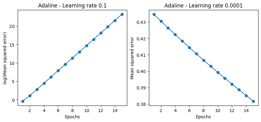
import os, urllib.request
os.makedirs('figures', exist_ok=True)
fig_path = 'figures/02_12.png'
if not os.path.exists(fig_path):
    url = 'https://raw.githubusercontent.com/rasbt/machine-learning-book/main/ch02/figures/02_12.png'
    try:
        urllib.request.urlretrieve(url, fig_path)
    except Exception as e:
        print(f'Could not download figure: {e}')
if os.path.exists(fig_path):
    display(Image(filename=fig_path, width=700))
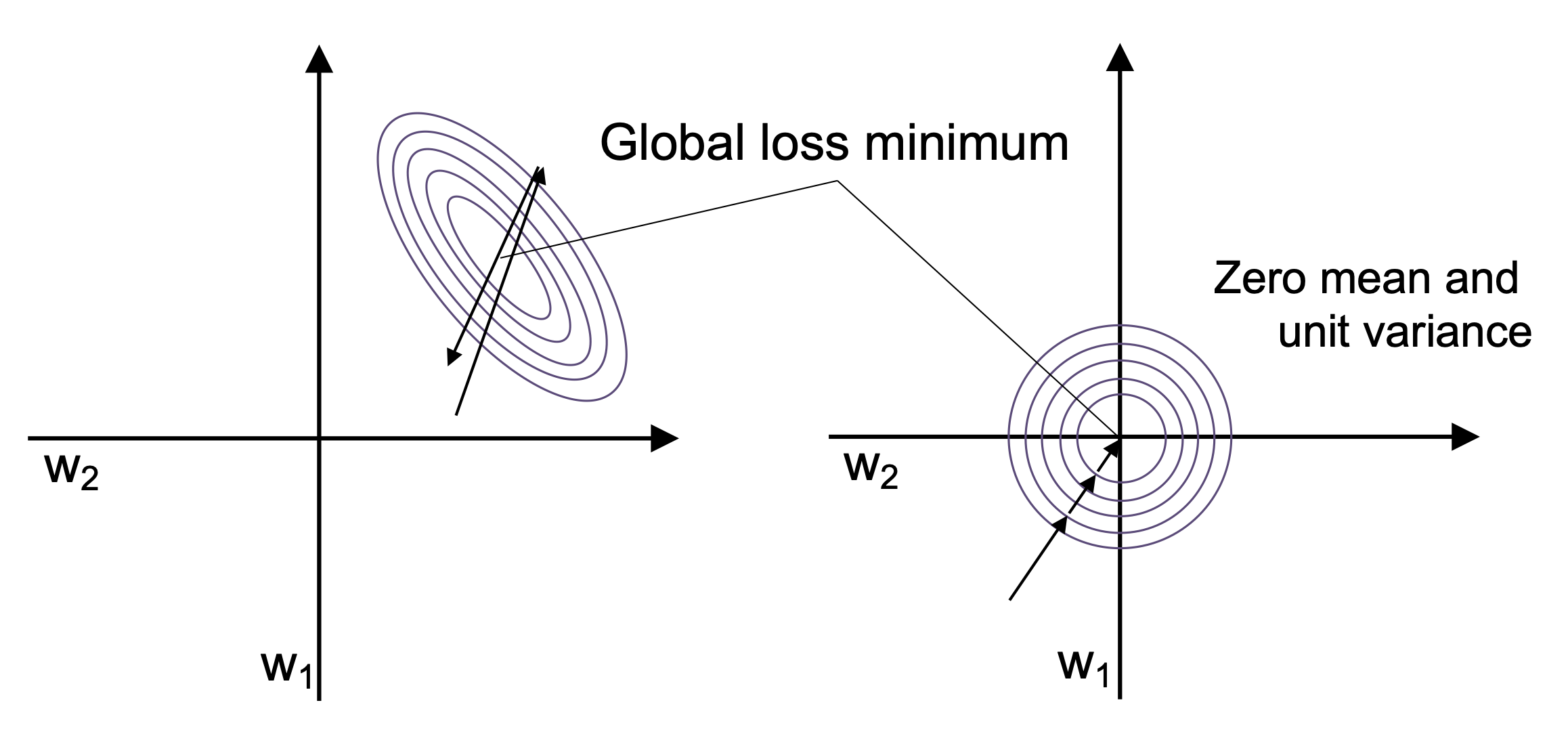
Improving gradient descent through feature scaling
import os, urllib.request
os.makedirs('figures', exist_ok=True)
fig_path = 'figures/02_13.png'
if not os.path.exists(fig_path):
    url = 'https://raw.githubusercontent.com/rasbt/machine-learning-book/main/ch02/figures/02_13.png'
    try:
        urllib.request.urlretrieve(url, fig_path)
    except Exception as e:
        print(f'Could not download figure: {e}')
if os.path.exists(fig_path):
    display(Image(filename=fig_path, width=700))
# standardize features
X_std = np.copy(X)
X_std[:, 0] = (X[:, 0] - X[:, 0].mean()) / X[:, 0].std()
X_std[:, 1] = (X[:, 1] - X[:, 1].mean()) / X[:, 1].std()
ada_gd = AdalineGD(n_iter=20, eta=0.5)
ada_gd.fit(X_std, y)
plot_decision_regions(X_std, y, classifier=ada_gd)
plt.title('Adaline - Gradient descent')
plt.xlabel('Sepal length [standardized]')
plt.ylabel('Petal length [standardized]')
plt.legend(loc='upper left')
plt.tight_layout()
#plt.savefig('images/02_14_1.png', dpi=300)
plt.show()
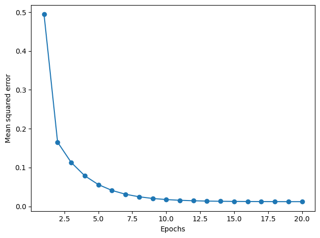
plt.plot(range(1, len(ada_gd.losses_) + 1), ada_gd.losses_, marker='o')
plt.xlabel('Epochs')
plt.ylabel('Mean squared error')
plt.tight_layout()
#plt.savefig('images/02_14_2.png', dpi=300)
plt.show()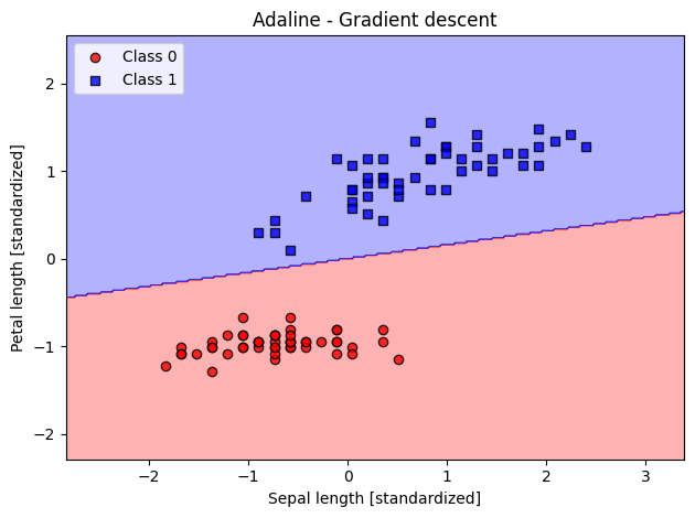
Large scale machine learning and stochastic gradient descent
The AdalineSGD class is an implementation of the Adaptive Linear Neuron (Adaline) algorithm. The Adaline algorithm is an extension of the perceptron algorithm, and is used to train a single-layer neural network to classify linearly separable data.
This implementation of Adaline uses Stochastic Gradient Descent (SGD) to update the weights, instead of batch gradient descent. This means that the weights are updated incrementally for each training example, rather than after evaluating the gradient over the entire training set.
The class has several attributes and methods:
Attributes:
eta: the learning rate (between 0.0 and 1.0)n_iter: the number of passes over the training datasetshuffle: whether to shuffle the training data every epoch (to prevent cycles)random_state: the seed for the random number generator used to initialize the weightsw_: the weights after fittingb_: the bias unit after fittinglosses_: the mean squared error loss function value averaged over all training examples in each epoch
Methods:
__init__: Initialize the object with default or user-specified values for the learning rate, number of iterations, and other parameters.fit: Fit the training data to the model.partial_fit: Fit the training data to the model without reinitializing the weights._shuffle: Shuffle the training data._initialize_weights: Initialize the weights to small random numbers._update_weights: Apply the Adaline learning rule to update the weights.net_input: Calculate the net input.activation: Compute linear activation.predict: Return the class label after the unit step.
class AdalineSGD:
    """ADAptive LInear NEuron classifier.

    Parameters
    ------------
    eta : float
      Learning rate (between 0.0 and 1.0)
    n_iter : int
      Passes over the training dataset.
    shuffle : bool (default: True)
      Shuffles training data every epoch if True to prevent cycles.
    random_state : int
      Random number generator seed for random weight
      initialization.


    Attributes
    -----------
    w_ : 1d-array
      Weights after fitting.
    b_ : Scalar
        Bias unit after fitting.
    losses_ : list
      Mean squared error loss function value averaged over all
      training examples in each epoch.


    """
    def __init__(self, eta=0.01, n_iter=10, shuffle=True, random_state=None):
        self.eta = eta
        self.n_iter = n_iter
        self.w_initialized = False
        self.shuffle = shuffle
        self.random_state = random_state

    def fit(self, X, y):
        """ Fit training data.

        Parameters
        ----------
        X : {array-like}, shape = [n_examples, n_features]
          Training vectors, where n_examples is the number of examples and
          n_features is the number of features.
        y : array-like, shape = [n_examples]
          Target values.

        Returns
        -------
        self : object

        """
        self._initialize_weights(X.shape[1])
        self.losses_ = []
        for i in range(self.n_iter):
            if self.shuffle:
                X, y = self._shuffle(X, y)
            losses = []
            for xi, target in zip(X, y):
                losses.append(self._update_weights(xi, target))
            avg_loss = np.mean(losses)
            self.losses_.append(avg_loss)
        return self

    def partial_fit(self, X, y):
        """Fit training data without reinitializing the weights"""
        if not self.w_initialized:
            self._initialize_weights(X.shape[1])
        if y.ravel().shape[0] > 1:
            for xi, target in zip(X, y):
                self._update_weights(xi, target)
        else:
            self._update_weights(X, y)
        return self

    def _shuffle(self, X, y):
        """Shuffle training data"""
        r = self.rgen.permutation(len(y))
        return X[r], y[r]

    def _initialize_weights(self, m):
        """Initialize weights to small random numbers"""
        self.rgen = np.random.RandomState(self.random_state)
        self.w_ = self.rgen.normal(loc=0.0, scale=0.01, size=m)
        self.b_ = np.float64(0.)
        self.w_initialized = True

    def _update_weights(self, xi, target):
        """Apply Adaline learning rule to update the weights"""
        output = self.activation(self.net_input(xi))
        error = (target - output)
        self.w_ += self.eta * 2.0 * xi * (error)
        self.b_ += self.eta * 2.0 * error
        loss = error**2
        return loss

    def net_input(self, X):
        """Calculate net input"""
        return np.dot(X, self.w_) + self.b_

    def activation(self, X):
        """Compute linear activation"""
        return X

    def predict(self, X):
        """Return class label after unit step"""
        return np.where(self.activation(self.net_input(X)) >= 0.5, 1, 0)
import os
os.makedirs('figures', exist_ok=True)
ada_sgd = AdalineSGD(n_iter=15, eta=0.01, random_state=1)
ada_sgd.fit(X_std, y)
plot_decision_regions(X_std, y, classifier=ada_sgd)
plt.title('Adaline - Stochastic gradient descent')
plt.xlabel('Sepal length [standardized]')
plt.ylabel('Petal length [standardized]')
plt.legend(loc='upper left')
plt.tight_layout()
plt.savefig('figures/02_15_1.png', dpi=300)
plt.show()
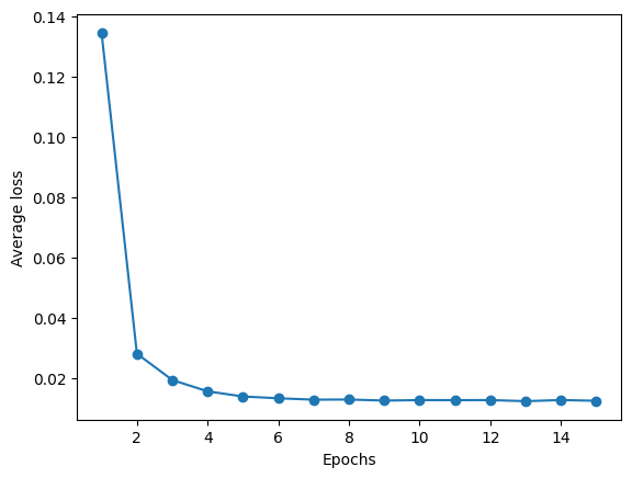
plt.plot(range(1, len(ada_sgd.losses_) + 1), ada_sgd.losses_, marker='o')
plt.xlabel('Epochs')
plt.ylabel('Average loss')
plt.savefig('figures/02_15_2.png', dpi=300)
plt.show()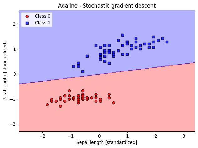
ada_sgd.partial_fit(X_std[0, :], y[0])<__main__.AdalineSGD at 0x7a67b26134a0>Summary
...
Readers may ignore the following cell